Sensitivity and identifiability of rheological parameters in debris flow modeling

Over the past decades, several numerical models have been developed to understand, simulate and predict debris flow events. Typically, these models simplify the complex interactions between water and solids using a single-phase approach and different rheological models to represent flow resistance. In this study, we perform a sensitivity analysis on the parameters of a debris flow numerical model (FLO-2D) for a suite of relevant variables (i.e., maximum flood area, maximum flow velocity, maximum height and deposit volume). Our aims are to (i) examine the degree of model overparameterization and (ii) assess the effectiveness of observational constraints to improve parameter identifiability. We use the Distributed Evaluation of Local Sensitivity Analysis (DELSA) method, which is a hybrid local–global technique. Specifically, we analyze two creeks in northern Chile (∼29^∘ S, 70^∘ W) that were affected by debris flows on 25 March 2015. Our results show that SD (surface detention) and β₁ (a parameter related to viscosity) provide the largest sensitivities. Further, our results demonstrate that equifinality is present in FLO-2D and that the final deposited volume and maximum flood area contain considerable information to identify model parameters.

1 Introduction

In steep mountain environments, intense and localized storms can trigger the sudden movement of sediments, generating flash floods with solid volumetric concentrations up to 40 %–60 % (Takahashi, 1981; O'Brien and Julien, 1988; Calvo and Savi, 2009). These events, also known as debris flows, differ from water floods because – in addition to fluid stress – solid–fluid and solid–solid interactions dominate the flow motion (Takahashi, 1981; Iverson et al., 1997). In recent years, debris flows have been recognized as a major natural hazard (Calvo and Savi, 2009), affecting infrastructure, economic activities and human life. For instance, debris flow events in Switzerland produced 24 fatalities and overall losses of USD 380 million during the period 1972–2007 (Hilker et al., 2009). In Chile, estimated economic losses associated with the five biggest debris flow events recorded over 1980–2017 were at least USD 1.6 billion with nearly 1000 people dead or missing (Servicio Nacional de Geología y Minería, 2017).

Over the last decades, numerical models have emerged as a powerful tool to understand the behavior and magnitude of debris flow events, since they allow for the quantification of key variables used by engineers and decision-makers for risk management (Quan Luna et al., 2011; Frey et al., 2016; Calvo and Savi, 2009) and urban planning (Hürlimann et al., 2006; Lucà et al., 2014; Naef et al., 2006; Arattano et al., 2006). However, the application of debris flow models requires several assumptions and simplifications that make results diverge from reality at various levels (Sosio et al., 2007). For example, uncertainties in terrain elevation models (e.g., satellite product and horizontal resolution), physical parameters (e.g., rheology parameters and solid concentration) and hydrological fluxes (e.g., precipitation and streamflow) used to force debris flow simulations can substantially impact relevant variables, such as flood area, sediment volumes or maximum flow depth.

The use of debris flow models for practical problems typically requires the implementation of single-phase numerical models (Rickenmann et al., 2006; Naef et al., 2006) that solve one-dimensional or two-dimensional Saint Venant equations, using different rheological approaches to account for frictional stress S_f. Many studies have reported good agreement between debris flow model results and post-event measurements, e.g., runout distance, flow velocity, deposit depth and flood area (D'Agostino and Tecca, 2006; Naef et al., 2006; Sosio et al., 2007; Rickenmann et al., 2006; Cesca and D'Agostino, 2008; Lin et al., 2011; Hungr, 1995). Nevertheless, it is recognized that, because complex debris flow dynamics change in time and space (Coussot and Meunier, 1996), the appropriate choice of rheological parameters is critical for a good agreement between debris flow model output and field data (Sosio et al., 2007). In this context, various approaches have been adopted to characterize the sensitivity of debris flow model results to variations in model parameters, i.e., the coefficients in the model equations. For example, D'Agostino and Tecca (2006) compared FLO-2D (O'Brien and Garcia, 2009) simulations performed with two sets of rheological parameters and three values of the laminar coefficient K (six simulations in total), concluding that K controls the flood area and that rheological parameters control the maximum depth. Boniello et al. (2010) compared FLO-2D model results from a set of 12 back-calculated rheological parameters selected from previous studies, with another set of parameter values obtained from laboratory rheological analyses, finding a better representation of debris flow behavior with back-calculated parameters. Chow et al. (2018) conducted simulations with FLO-2D using 26 different sets of rheological parameters obtained from previous studies, combined with different values of volumetric sediment concentration C_v, specific gravity G_s and the surface detention SD, a parameter used in FLO-2D to represent flow detention. They found that the most important parameters were C_v, SD and β₁, which characterizes fluid viscosity. All these studies used fixed sets of rheological parameters in their numerical experiments, and, therefore, the relative importance of such coefficients on relevant simulated variables – specifically, flow depth, flow velocity, deposit volume and flood area – remains unknown. Therefore, this paper addresses the following questions:

1. How sensitive are debris flow model results to uncertain – and typically fixed – rheological parameters?

2. What are the most effective post-event measurements to constrain the parameter search towards more realistic simulations?

To answer these questions, we perform a sensitivity analysis on the parameters of a numerical debris flow model and examine the effects of using post-event in situ measurements on expected parameter ranges. In particular, we analyze a debris flow event that occurred in two creeks located in the Atacama region (northern Chile; ∼29^∘ S, 70^∘ W) during March 2015. This event was the consequence of heavy precipitation over a 3 d period, which exceeded 60 mm at several locations (Bozkurt et al., 2016), resulting in the loss of human lives and massive infrastructure damage. Therefore, our intention is to provide guidance on the choice of uncertain rheological parameters, contributing to more reliable numerical simulations for debris flow risk assessments and land use planning. The remainder of this paper is organized as follows: Sect. 2 describes the case study creeks and data; Sect. 3 describes the numerical debris flow model, sensitivity analysis and parameter search strategies; Sect. 4 presents the results and discussion; and Sect. 5 summarizes our main findings.

2 Study domain and data

We choose two ephemeral creeks located nearby in the upper Huasco River basin, Acerillas and La Mesilla (Fig. 1a), where debris flows were triggered by an extreme precipitation event on 24–26 March 2015 (Bozkurt et al., 2016; Ortega et al., 2019). The Huasco Valley is a semi-arid fluvial system located at the southern edge of the Atacama region, Chile. This valley is characterized by perennial rivers that only exist in the trunk valleys, while tributaries only show ephemeral streams. In these areas, heavy rainfall events may induce catastrophic debris flows and mud floods that greatly contribute to erosion (Aguilar et al., 2020).

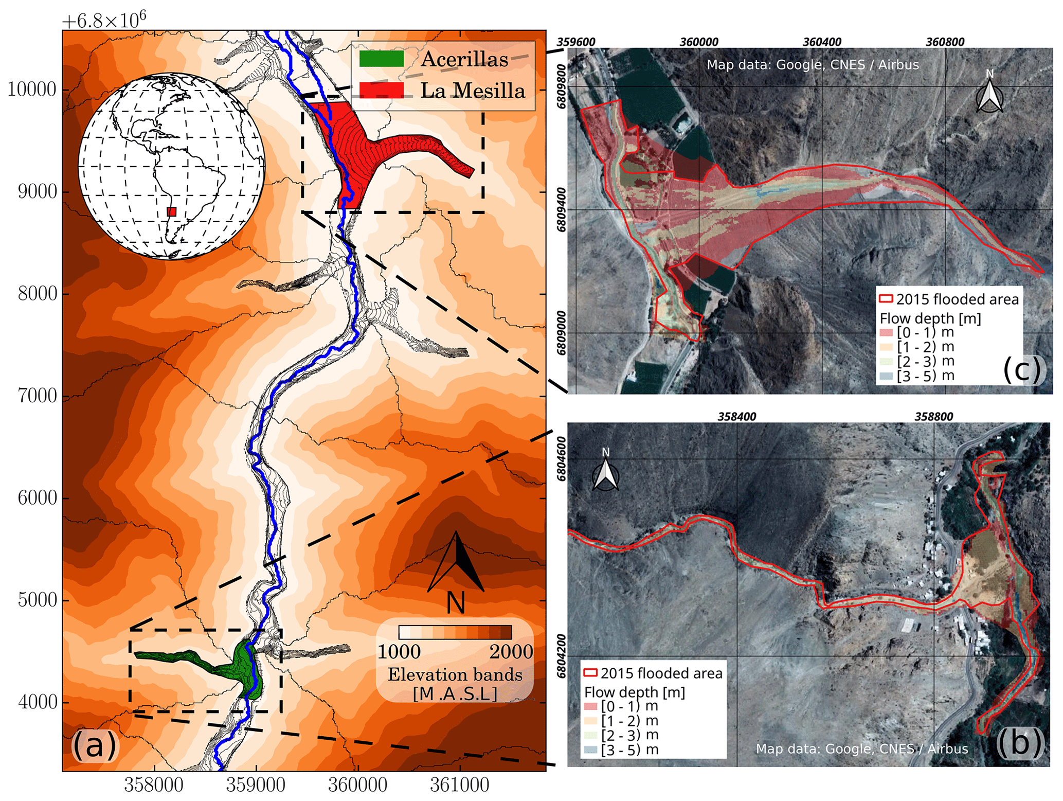
Figure 1 (a) Location of the two case study creeks and reference model results. The maximum observed flood areas and modeled flow depth (reference models) are shown for (b) Acerillas creek and (c) La Mesilla creek. Elevations bands created from a satellite digital elevation model (DEM) at 12×12 m: © JAXA/METI ALOS PALSAR L1.0 2007 (Japan Aerospace Exploration Agency/Ministry of Economy, Trade and Industry Advanced Land Observing Satellite Phased Array type L-band Synthetic Aperture Radar). Accessed through the ASF DAAC (Alaska Satellite Facility Distributed Active Archive Center) on 11 June 2017.

The Acerillas creek (15 km² basin area; Fig. 1b) has a markedly narrow channel with almost no alluvial fan, allowing for the transportation of sediments towards the El Carmen River. Post-event measurements indicate a deposited sediment volume of 6000 m³ (Cabré et al., 2020) and a maximum flood area of 37 000 m². Conversely, the La Mesilla creek (2.5 km² basin area; Fig. 1c) is characterized by a big alluvial fan where considerable sedimentation occurs, and post-event measurements show a deposited sediment volume of 102 000 m³ (Cabré et al., 2020) and a maximum flood area of 246 500 m². These flood areas were estimated by comparing pre- and post-event satellite Google Earth imagery. Also, a post-event topography lidar scan (acquired in February–March 2017 by the Chilean Ministry of Public Works) was available for this study. This dataset has a 1×1 m² horizontal resolution and was post-processed in order to eliminate vegetation and buildings.

Flow discharge data at the outlet of each creek were obtained from a distributed hydrological model, HEC-HMS (Hydrologic Engineering Center Hydrologic Modeling System) version 4.2 (USACE, 2015). The model was configured for the entire Huasco River basin (7242 km²), upstream of the Santa Juana irrigation reservoir, as part of a debris flow mitigation project for the Chilean Ministry of Public Works. Hydrologic model simulations were forced using data from point measurements at 14 meteorological stations, spatially distributed with the inverse-distance-weighting (IDW) interpolation method (Teegavarapu et al., 2006). Total rainfall records range from 20 to 76 mm, with a maximum registered intensity of 16 mm h⁻¹. The HEC-HMS model parameters were calibrated against hourly streamflow observed at two gauge stations located in the upper part of the basin – Río El Carmen en El Corral and Río Conay en Las Lozas (Fig. 2) – obtaining a Nash–Sutcliffe efficiency (NSE; Nash and Sutcliffe, 1970) of 0.78 for the former and 0.64 for the latter. Although all the other gauging stations were buried or destroyed by debris flows, simulated total water volumes were similar with those captured by the Santa Juana reservoir, whose levels were low before the event. Estimated peak flow discharges for the event analyzed are 8 m³ s⁻¹ at La Mesilla and 12.7 m³ s⁻¹ at Acerillas.

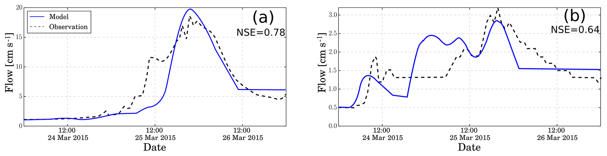
Figure 2 Calibration records for stream gauge stations (a) Río El Carmen en El Corral and (b) Río Conay en Las Lozas.

3 Methods

3.1 Debris flow model

We use the two-dimensional FLO-2D debris flow model (O'Brien et al., 1993), configured at a 10 m horizontal resolution. FLO-2D is a finite difference model that simulates water or debris flows in channels or unconfined surfaces. The governing equations solved by FLO-2D are the depth-averaged continuity and momentum conservation (Eqs. 1 and 2), and the flood wave progression is controlled by topography and flow resistance (O'Brien and Julien, 1988). FLO-2D can also simulate debris flow rheologies using a “quadratic” rheological model that combines components associated with creep, viscous, dispersive (collisions) and turbulent stresses (O'Brien and Julien, 1988; O'Brien and Garcia, 2009; Naef et al., 2006). Based on this quadratic rheology, the friction slope S_f is estimated as (Eq. 3):

$$\begin{array}{}\text{(1)}& {\displaystyle }{\displaystyle \frac{\partial h}{\partial t}}+{\displaystyle \frac{\partial h{V}_x}{\partial x}}+{\displaystyle \frac{\partial h{V}_y}{\partial y}}=\mathrm{0},\text{(2)}& {\displaystyle }\begin{array}{rl}& S_{{\mathrm{f}}_x}=S_{{\mathrm{o}}_x}-{\displaystyle \frac{\partial h}{\partial x}}-{\displaystyle \frac{V_x}{g}}{\displaystyle \frac{\partial V_x}{\partial x}}-{\displaystyle \frac{V_y}{g}}{\displaystyle \frac{\partial V_x}{\partial y}}-{\displaystyle \frac{\mathrm{1}}{g}}{\displaystyle \frac{\partial V_x}{\partial t}}\\ & S_{{\mathrm{f}}_y}=S_{{\mathrm{o}}_y}-{\displaystyle \frac{\partial h}{\partial y}}-{\displaystyle \frac{V_y}{g}}{\displaystyle \frac{\partial V_y}{\partial y}}-{\displaystyle \frac{V_x}{g}}{\displaystyle \frac{\partial V_y}{\partial x}}-{\displaystyle \frac{\mathrm{1}}{g}}{\displaystyle \frac{\partial V_y}{\partial t}},\end{array}\text{(3)}& {\displaystyle }{S}_{\mathrm{f}}={\displaystyle \frac{{\mathit{\tau }}_{\mathrm{y}}}{{\mathit{\gamma }}_{m}h}}+{\displaystyle \frac{K\mathit{\eta }V}{\mathrm{8}{\mathit{\gamma }}_m{h}^{\mathrm{2}}}}+{\displaystyle \frac{n_{\mathrm{td}}^{\mathrm{2}}{V}^{\mathrm{2}}}{h^{\mathrm{3}/\mathrm{4}}}},\end{array}$$

where h is the local flow depth, t is time, V_x and V_y are depth-averaged velocity components along the x and y directions, g is gravitational acceleration, S_f is the friction slope, S_o is the bed slope, τ_y is the yield stress, K is a laminar strength parameter, η is the interstitial fluid dynamic viscosity, and n_td is the conventional Manning's roughness coefficient corrected by C_v ($n_{\mathrm{td}}=\mathrm{0.0538}n{e}^{\mathrm{6.0896}{C}_{\mathrm{v}}}$; O'Brien and Julien, 1988). O'Brien et al. (1993) proposed the following empirical relationships to calculate the viscosity and yield stress as a function of the volumetric sediment concentration c_v (Eqs. 4 and 5):

$$\begin{array}{}\text{(4)}& {\displaystyle }& {\displaystyle }\mathit{\eta }={\mathit{\alpha }}_{\mathrm{1}}{e}^{{\mathit{\beta }}_{\mathrm{1}}{c}_{\mathrm{v}}},\text{(5)}& {\displaystyle }& {\displaystyle }{\mathit{\tau }}_{\mathrm{y}}={\mathit{\alpha }}_{\mathrm{2}}{e}^{{\mathit{\beta }}_{\mathrm{2}}{c}_{\mathrm{v}}},\end{array}$$

where α_1,2 and β_1,2 are experimentally defined empirical coefficients (O'Brien et al., 1993; O'Brien and Garcia, 2009).

3.2 Sensitivity analysis

Sensitivity analysis (SA) is a powerful tool to characterize the effects of variations in input factors on environmental-model responses (Razavi and Gupta, 2015; Gupta and Razavi, 2018). When the factors of interest are the model parameters, SA helps to identify those that are redundant for the modeling purposes, contributing to a more efficient parameter search (Mendoza et al., 2015). Different types of SA techniques have been proposed in the literature depending on specific objectives or even the meaning of sensitivity (see, for example, reviews by Razavi and Gupta, 2015, and Pianosi et al., 2016).

In this work, we apply the Distributed Evaluation of Local Sensitivity Analysis (DELSA) method (Rakovec et al., 2014), which is a frugal local–global hybrid technique, to identify the parameters that have the largest impact on simulated debris flow variables. Although our implementation only examines first-order sensitivities across the parameter space – as in Rakovec et al. (2014) – it should be noted that DELSA has considerable unexplored potential to characterize parameter interactions, which could be achieved by including additional terms in the prediction total variance, as suggested by Sobol and Kucherenko (2010).

First-order sensitivities are obtained using local gradients that quantify the sensitivity of a modeled output Ψ relative to individual variations of a parameter θ_j. The local gradients $\frac{\partial \mathrm{\Psi }}{\partial {\mathit{\theta }}_j}{|}_k$ are used to compute the first-order sensitivity of each parameter j at each point k of the parameter space:

$$\begin{array}{}\text{(6)}& S{\mathrm{1}}_k^j={\displaystyle \frac{|\frac{\partial {\mathrm{\Psi }}_{kj}}{\partial {\mathit{\theta }}_j}{|}^{\mathrm{2}}\frac{\mathrm{1}}{\mathrm{12}}{\left({\mathit{\theta }}_{i,\max }-{\mathit{\theta }}_{i,\min }\right)}^{\mathrm{2}}}{V_K\left(\mathrm{\Psi }\right)}},\end{array}$$

where V_K(Ψ) is the total local variance at point k

$$\begin{array}{}\text{(7)}& V_K\left(\mathrm{\Psi }\right)=\sum _{j=\mathrm{0}}^J|{\displaystyle \frac{\partial {\mathrm{\Psi }}_{kj}}{\partial {\mathit{\theta }}_j}}{|}^{\mathrm{2}}{\displaystyle \frac{\mathrm{1}}{\mathrm{12}}}{\left({\mathit{\theta }}_{i,\max }-{\mathit{\theta }}_{i,\min }\right)}^{\mathrm{2}}.\end{array}$$

The first-order sensitivity measures $S{\mathrm{1}}_k^j$ vary between 0 and 1, and the sum of first-order sensitivities from all parameters is equal to 1 at each sample point. In this work, parameter sampling is performed using the Latin hypercube sampling (LHS) method. LHS is a statistical method to generate an almost random sample of parameter values from a multidimensional distribution and has proven to be more efficient than other methods like Monte Carlo sampling (Olsson et al., 2003; Olsson and Sandberg, 2002).

Local sensitivities can be analyzed in a disaggregated manner – through their cumulative frequency distribution across the parameter space – or aggregated by computing a specific statistical property, e.g., the median of all local sensitivity measures for a particular pair of parameter and target variables. We use both approaches to analyze SA results.

In this paper, we focus on the effects of debris flow model parameters on four response variables: maximum average runoff speed V_mean (m s⁻¹), maximum average runoff height H_mean (m), maximum flood area A_max (m²) and deposited volume Vol_dep (m³). These response variables are calculated using the outputs from FLO-2D as

$$\begin{array}{}\text{(8)}& {\displaystyle }& {\displaystyle }{V}_{\mathrm{mean}}=\sum _{j=\mathrm{0}}^{N_{\mathrm{WC}}}{V}_{\max }\left(j\right)/N_{\mathrm{WC}},\text{(9)}& {\displaystyle }& {\displaystyle }{H}_{\mathrm{mean}}=\sum _{j=\mathrm{0}}^{N_{\mathrm{WC}}}{H}_{\max }\left(j\right)/N_{\mathrm{WC}},\end{array}$$

$$\begin{array}{}\text{(10)}& {\displaystyle }& {\displaystyle }{A}_{\max }=\sum _{j=\mathrm{0}}^{N_{\mathrm{WC}}}\mathrm{d}x\cdot \mathrm{d}y,\text{(11)}& {\displaystyle }& {\displaystyle }{\mathrm{Vol}}_{\mathrm{dep}}=\sum _{j=\mathrm{0}}^{N_{\mathrm{WC}}}{H}_{\mathrm{final}}\left(j\right)\mathrm{d}x\cdot \mathrm{d}y,\end{array}$$

where j is the cell index; N_WC is the total number of wet cells (h>0); dx and dy indicate the cell size along the x and y axis (numerical grid); and V_max(j), H_max(j) and H_final(j) are the maximum flow speed, maximum flow depth and final runoff height of the cell j, respectively.

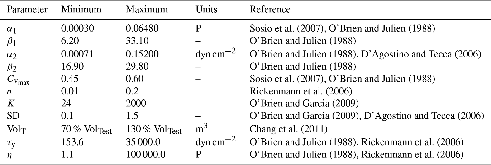
The FLO-2D parameters considered for DELSA are those that describe the fluid rheology (Table 1): α_1,2, β_1,2, C_v, K, n, the SD parameter and the total volume of sediments mobilized Vol_T.

The detention coefficient SD is a model parameter that controls flow detention. The FLO-2D user's manual and previous studies (D'Agostino and Tecca, 2006) suggest that SD acts as the minimum physically plausible flow depth (i.e., flow stops if flow depth < SD). Further, D'Agostino and Tecca (2006) noted that this coefficient has a strong influence on the results, and it can be used as a surrogate of the rheology. The estimated total sediment volume mobilized Vol_Test by each debris flow event was calculated with the equation proposed by Chang et al. (2011) (Eq. 12).

$$\begin{array}{}\text{(12)}& \begin{array}{rl}{\mathrm{Vol}}_{\mathrm{Test}}& =\mathrm{0.023}{A}_{\mathrm{w}}+\mathrm{0.064}{A}_{\mathrm{L}}+\mathrm{13264.6}\mathrm{GI}-\mathrm{1399.2}D\\ & +\mathrm{38.47}{C}_{\mathrm{R}},\end{array}\end{array}$$

where A_w is the watershed area, A_L is the landslide area (zero in these cases), GI is the geological index (where a value of 2.5 is assumed based on a study zone report made for the Chilean Ministry of Public Works), D is the rainfall duration (D=48 h for this event) and C_R is the cumulative rainfall (C_R=76 mm). We obtain Vol_Test values of 185 000 m³ for Acerillas and 154 000 m³ for La Mesilla.

Debris flow concentration is assumed to vary with streamflow between a minimum concentration $C_{{\mathrm{v}}_{\min }}=\mathrm{0.1}$–0.4 and a maximum concentration $C_{{\mathrm{v}}_{\max }}$ at the time of peak flow, which is treated as a model parameter. To this end, we propose the following function for C_v:

$$\begin{array}{}\text{(13)}& \begin{array}{rl}& C_{\mathrm{v}}\left(t\right)=\\ & \left\{\begin{array}{ll}\frac{\left(C_{{\mathrm{v}}_{\max }}-C_{{\mathrm{v}}_{\min }}\right)\cdot \mathrm{erf}\left(\left(Q\left(t\right)-Q_m\right)/\left(Q_{\max }-Q_m\right)\cdot \mathit{\varphi }\right)\cdot \left(C_{{\mathrm{v}}_{\max }}-C_{{\mathrm{v}}_{\min }}\right)}{\left(\left(C_{{\mathrm{v}}_{\max }}-C_{{\mathrm{v}}_{\min }}\right)\cdot \mathrm{erf}\left(\left(Q_{\max }-Q_m\right)/\left(Q_{\max }-Q_m\right)\cdot \mathit{\varphi }\right)\right)}+C_{{\mathrm{v}}_{\min }},& \mathrm{if}Q\left(t\right)/Q_{\mathrm{mean}}\ge \mathrm{0.5}\\ C_{{\mathrm{v}}_{\min }},& \mathrm{if}Q\left(t\right)/Q_{\mathrm{mean}}<\mathrm{0.5},\end{array}\right.\end{array}\end{array}$$

where ϕ is a coefficient that changes the shape of the concentration curve. ϕ and $C_{{\mathrm{v}}_{\min }}$ are calculated in order to match the total volume and minimize $C_{{\mathrm{v}}_{\min }}$ value:

$$\begin{array}{}\text{(14)}& \begin{array}{ll}\text{minimize}& C_{{\mathrm{v}}_{\min }}\\ \mathrm{subject}\mathrm{to}& {\int }_{t=\mathrm{0}}^{\mathrm{T}}{C}_{\mathrm{v}}\left(t\right)\cdot Q\left(t\right)\cdot \mathrm{d}t={\mathrm{Vol}}_{\mathrm{T}}.\end{array}\end{array}$$

Rheological parameter ranges are obtained from previous debris flow studies (O'Brien and Julien, 1988; Boniello et al., 2010; D'Agostino and Tecca, 2006; Sosio et al., 2007; Rickenmann et al., 2006; Chang et al., 2011; O'Brien and Garcia, 2009) and are summarized in Table 1. However, additional restrictions are imposed for τ_y and η, with maximum values of 35 000 dyn cm⁻² (dyne; g cm s⁻²) and 100 000 P (poise; 0.1 kg m⁻¹ s⁻¹), respectively (Rickenmann et al., 2006). Since τ_y and η are functions of rheological parameters (Eqs. 5 and 4), such limits impose restrictions for α_1,2, β_1,2 and $C_{{\mathrm{v}}_{\max }}$ that we ensure are implemented in DELSA. To this end, we develop a Python script that allows for running FLO-2D in parallel and sequentially, reducing computational cost considerably. For Vol_T, we assume a range of variation of ±30 % with respect to estimated values (Eq. 12).

Sosio et al. (2007)O'Brien and Julien (1988)O'Brien and Julien (1988)O'Brien and Julien (1988)D'Agostino and Tecca (2006)O'Brien and Julien (1988)Sosio et al. (2007)O'Brien and Julien (1988)Rickenmann et al. (2006)O'Brien and Garcia (2009)O'Brien and Garcia (2009)D'Agostino and Tecca (2006)Chang et al. (2011)O'Brien and Julien (1988)Rickenmann et al. (2006)O'Brien and Julien (1988)Rickenmann et al. (2006)

Table 1 Values range of the model parameters. P: poise; dyn: dyne.

3.3 Parameter selection via constrained search

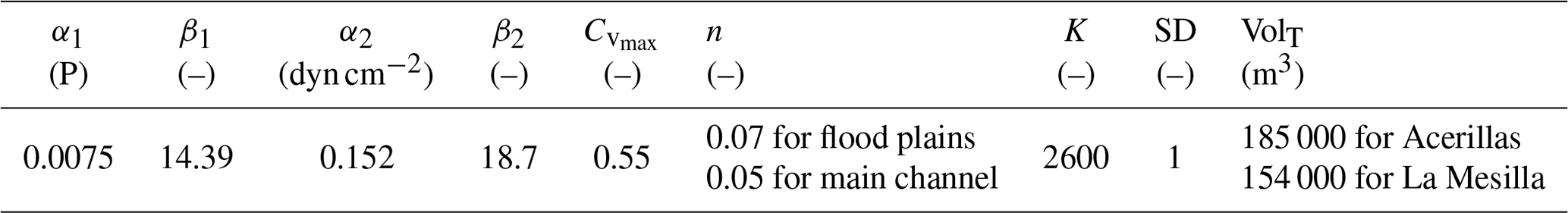
We explore the effects of parameter uncertainty on simulated debris flow variables at the two case study creeks. We also examine the utility of using reference values for specific variables to constrain the search of physically plausible parameter sets. Such values are obtained from a reference simulation conducted by Zegers (2017), who reproduced flood area and sediment volume observed during the 2015 debris flow events at Acerillas and La Mesilla creeks using FLO-2D. Zegers (2017) calibrated model parameters by contrasting results against measured flood areas, deposited volumes and flow velocity estimated from a video captured with a cell phone by a local person at Acerillas. Such a validation strategy has provided reliable results for several other creeks in the area. Parameter values used for the reference simulation are provided in Table 2. Modeled flood areas and maximum flow depth are shown in Fig. 1, and discrepancies with respect to observations can be attributed to the use of post-event topography.

Based on the reference simulation, we choose reference values of V_mean=1 m s⁻¹ and H_mean=1.5 m at both creeks. Additionally, we estimate the reference maximum flood area using Google Earth imagery – obtaining values of 246 500 m² for La Mesilla and 37 000 m² for Acerillas – and use deposited sediment volumes reported by Cabré et al. (2020) as reference values, which correspond to 102 000 and 6000 m³ for La Mesilla and Acerillas, respectively.

Table 2 Parameter values for reference models on Zegers (2017). P: poise; dyn: dyne.

4 Results and discussion

4.1 Choice of sample size

First, we seek to identify the minimum sample size N_k for which stable DELSA results can be obtained in order to minimize computational cost (Rakovec et al., 2014). Therefore, we explore the effects of the choice of N_k on the cumulative frequency distributions (CDFs) of DELSA first-order sensitivity indices. Since we include N_j=9 parameters, the total number of simulations required for each case is $N_{\mathrm{t}}=(N_j+\mathrm{1})N_k$. Figure 3 illustrates the sensitivity of DELSA results to variations in sample size N_k for four variables simulated by FLO-2D, with respect to parameters β₁ and $C_{{\mathrm{v}}_{\max }}$, at the Acerillas creek. Since the curves obtained for N_k=500 and N_k=1000 show slight differences, departing from the CDF for N_k=100, we conclude that a sample size of N_k=500 is adequate for further analyses. The sensitivity of DELSA results to N_k was also examined at La Mesilla creek, obtaining the same conclusion regarding sample size (not shown).

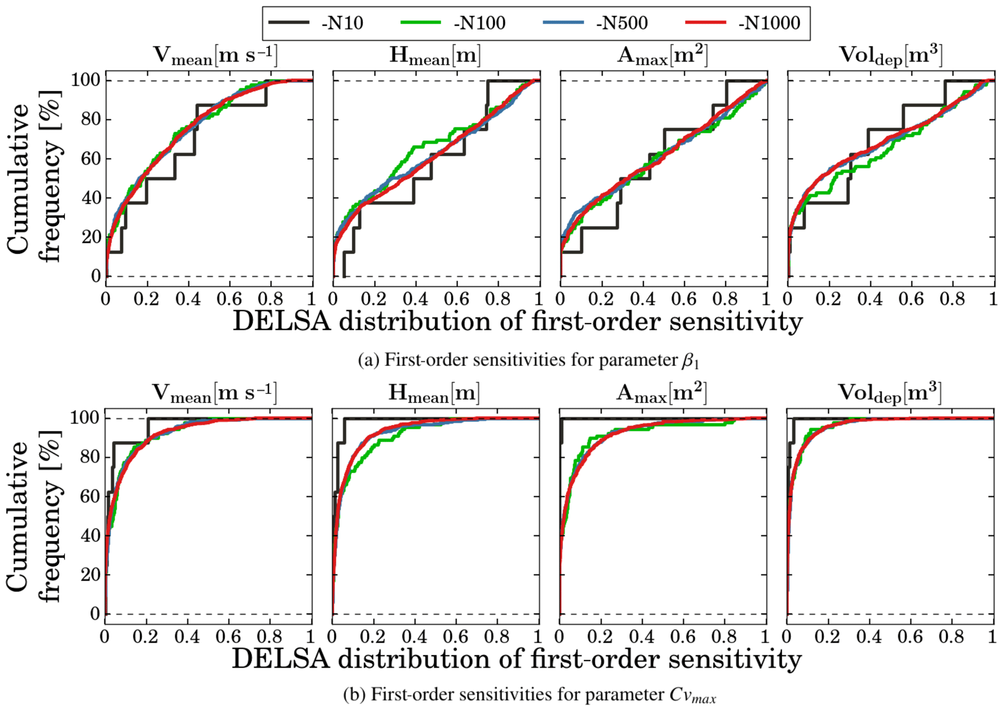
Figure 3 Effects of sample size N_k on the cumulative distribution function (CDF) of DELSA indices for parameters β₁ (a) and $C_{{\mathrm{v}}_{\max }}$ (b) at the Acerillas creek.

Figure 3 also shows that, depending on the target variable and parameter analyzed, first-order sensitivity indices can be highly heterogeneous across the parameter space. In particular, the modeled response is highly sensitive to variations of β₁, with first-order sensitivities larger than 0.2 for approximately 60 % of cases and sensitivities greater than 0.5 for 20 %–40 % depending on the variable analyzed. On the other hand, the modeled variables are less sensitive to $C_{{\mathrm{v}}_{\max }}$ in most cases, with DELSA indices smaller than 0.1 for approximately 70 % of the parameter sets.

4.2 Sensitivity of model responses to model parameters

Figure 4 displays the median of the full frequency distribution (obtained with N_k=500) of local first-order sensitivity indices for the two study domains: (i) Acerillas creek (ACE) and (ii) La Mesilla creek (MES). The uncertainty bands are obtained by performing bootstrapping with replacement (resampled 1000 times). In general, β₁ provides the largest sensitivities for the simulated variables analyzed, which means that the fluid rheology, in particular the viscosity coefficient (η=η(β₁)), is a main parameter controlling flow behavior. Moreover, the results of Acerillas seem to be more sensitive than those obtained at La Mesilla with respect to β₁. This could be better explained when analyzed together with SD, the detention coefficient.

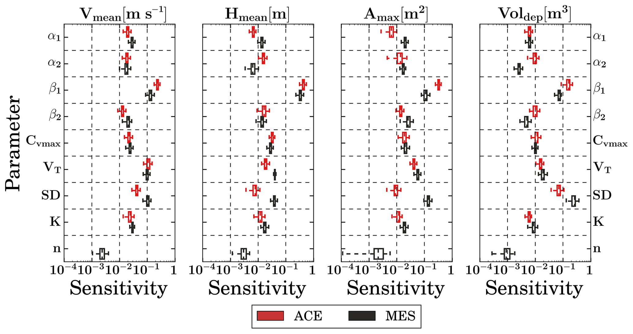
Figure 4 DELSA sensitivity indices (synthetized as the median from the cumulative frequency distribution) for all parameters and model responses. Results are displayed for Acerillas (red) and La Mesilla (black) creeks, and the sampling uncertainty (bootstrapping with 1000 times resampling) is indicated by boxplots. The vertical bold line in the boxplot is the median; the body of each boxplot shows the interquartile range (Q₇₅–Q₂₅); and the whiskers represent the sample minima and sample maxima. DELSA indices are displayed in log space for a better visualization of inter-parameter differences.

As expected, the simulated deposited volume Vol_dep is very sensitive to SD because this parameter controls flow detention. For the remaining simulated variables, SD also rises as an important parameter at La Mesilla, but it shows secondary importance at Acerillas, which can be explained by catchment differences. While the fluid rheology explains flow behavior at Acerillas creek (mainly sensitive to β₁), depositional or detention processes – represented by SD – gain importance across the larger alluvial fan of La Mesilla creek.

Another parameter that provides large sensitivities – especially in simulated mean flow velocity V_mean – is the total sediment volume Vol_T, whose sensitivities have the same order of magnitude as those produced by β₁. The high sensitivity of Vol_T on V_mean is explained because the former influences fluid rheology through C_v(t) (see Eqs. 4, 5 and 13). However, Vol_T does not produce large variations in the total deposited volume, which could be explained because, as deposition occurs, the flow is channelized between the deposited margins, preventing flow spreading. For example, when increasing SD values, A_max decreases as the flow is forced to stop at deeper heights. This could be a structural weakness of FLO-2D, which lacks proper representations of complex depositional and dewatering processes.

The large sensitivities in model response to variations of β₁ suggest that the viscous stress (second term in Eq. 3) is the main contributor to sensitivities in simulated frictional slope. On the other hand, DELSA sensitivity indices associated with yield stress τ_y and Manning's roughness coefficient – the other components of the frictional slope – are of second-order importance. Even more, model results are practically insensitive to Manning's roughness coefficient.

Our results show some differences with related previous work. D'Agostino and Tecca (2006) compared FLO-2D simulations performed with two sets of rheological parameters and three values of K (i.e., six simulations), concluding that the latter controls the flood area, while rheological parameters control the maximum flow depth. On the other hand, our results indicate that the laminar coefficient K provides small sensitivities in simulated flood areas and that the most influential rheological parameter on simulated maximum flow depth is β₁. Although D'Agostino and Tecca (2006) provided the first insights into FLO-2D parameter sensitivities, the number of parameters involved and the sample size were not large enough to draw robust conclusions. Recently, Chow et al. (2018) conducted simulations with FLO-2D using 26 different sets of rheological parameters obtained from 45 previous studies. They found that the most influential parameters – in order of importance – were C_v, SD and β₁. These results are different from ours due to discrepancies in the parameter sampling method, the use of fixed sets of rheological parameters and their parameter ranking definition, which does not consider separate effects on key simulated variables. For example, Chow et al. (2018) ignored the effect of the total sediment volume when analyzing C_v, whereas we examine the separate effects of maximum sediment concentration and total sediment volume, obtaining that the latter is more important than the maximum sediment concentration.

4.3 Parameter uncertainty effects

Figure 5 shows the full range of variation in model responses (produced by N_k=500 parameter sets), normalized by reference values obtained from post-event measurements (Vol_dep and A_max) and results obtained from the reference models (for H_mean and V_mean). These are compared with the simulated ensemble that results from screening model outputs imposing five different observational constraints: (i) ±20 % reference mean flow velocity (FVEL), (ii) ±20 % reference mean flow depth (FH), (iii) ±20 % reference maximum flood area (FAREA), (iv) ±40 % reference volume deposit (FVOL), and (v) ±20 % reference maximum flood area and ±40 % reference volume deposit (FAREAVOL). To be clear, constraint (i) results from keeping all those parameter sets that provide a simulated mean flow velocity within the range 0.8–1.2 V_ref. Constraints (ii)–(iv) work in a similar way for other observed variables, while constraint (v) filters all parameter sets that simultaneously provide flood areas and deposit volumes within the ranges 0.8–1.2 A_ref and 0.6–1.4 Vol_ref, respectively. We assume a weaker observational constraint in the case of the deposited volume because of possible uncertainties associated with different measurements techniques.

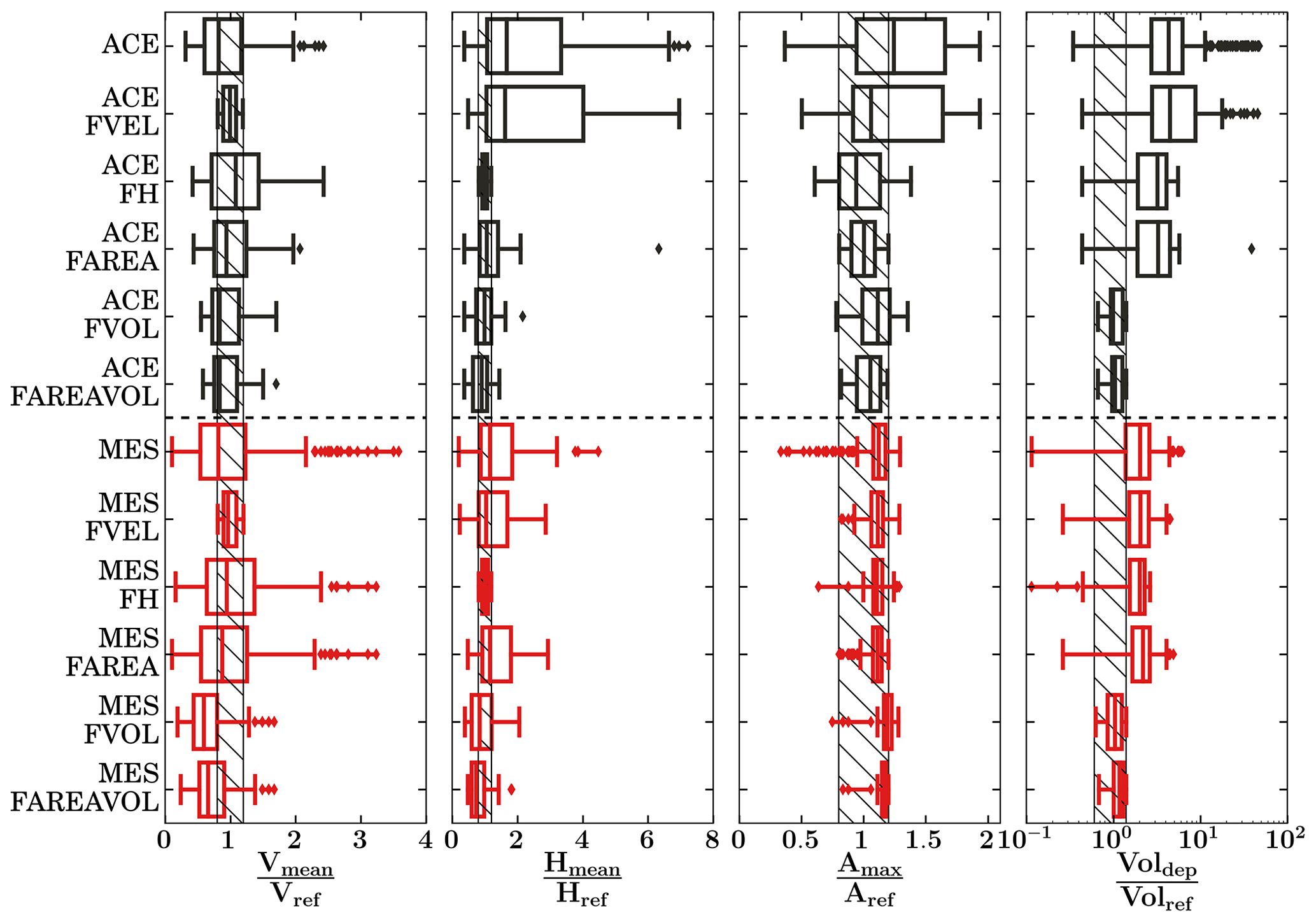
Figure 5 Effects of parametric uncertainty in normalized model responses for the original parameter sample (top panels) and alternative observational constraints – flow velocity (FVEL), flow depth (FH), flood area (FAREA) and sediment volume (FVOL) – and joint area–volume constraint (FAREAVOL). Results are displayed for Acerillas (black) and La Mesilla (red) creeks. The hatched area for V_mean, H_mean and A_max corresponds to ±20 % of their reference values, and for Vol_dep it is up to ±40 % of the estimated sediment volume. The vertical bold line in the boxplots is the median; the body of each boxplot shows the interquartile range (Q₇₅–Q₂₅); and the whiskers represent the sample minima and sample maxima.

Figure 5 also shows that, in general, the effects of parametric uncertainty on simulated variables are considerable and the ensemble median can be substantially different from the reference boundaries. This is somewhat expected, since the literature provides large ranges for model parameters (see Table 1 for details). Overall, uncertainties arising from the original parameter samples (top panels) are larger in Acerillas, except for mean flow velocity. This could be explained by the larger sensitivity of flow velocity to flow rheology, while the rest of simulated variables are more sensitive to deposition processes, mainly represented by SD.

Most simulations overestimate deposited volumes and flow depth, especially at Acerillas. For flow velocity, the ensemble of parameter sets provides mixed results in both creeks, with underestimation in most cases (median values lower than the reference values); however, there are still several parameter sets that produce an overestimation of flow velocity. The results obtained for maximum area reveal differences among both creeks: in Acerillas, most parameter sets tend to overestimate the flood area, whereas most simulated values are within the expected range at La Mesilla. This could happen because Vol_dep ≪ Vol_T at Acerillas, while Vol_dep ∼ Vol_T at La Mesilla; moreover, the maximum flood area at La Mesilla is approximately 6 times larger than in Acerillas. Thus, small variations in Vol_dep imply important fractional changes with respect to the volume reference values at Acerillas.

Figure 5 shows that the velocity constraint FVEL does not have an impact on the rest of simulated variables. Nevertheless, the application of alternative observational constraints helps to reduce the spread of the remaining variables. For example, the height filter FH improves simulations of maximum flood area, although it does not have much effect on velocity or deposit volume. The area restriction FAREA improves simulated flow depth only at Acerillas, as most of the original ensemble members were already inside the expected reference boundaries at La Mesilla. The volume constraint FVOL reduces the uncertainty in all variables, with the smallest improvement for flow velocity. This is because the volume is directly linked to flow height and flood area, but not to flow velocity. Finally, the largest reductions in ensemble spread are obtained when parameter sets are constrained by using area and volume observations (FAREAVOL).

The maximum flood area and deposited volume are relatively easy to measure and are probably the most used post-event measurements for calibrating debris flow models (Chow et al., 2018; Cesca and D'Agostino, 2008; D'Agostino and Tecca, 2006; Sosio et al., 2007; Frey et al., 2016; Quan Luna et al., 2011).

4.4 Parameter identifiability

Figure 6 illustrates the effects of applying observational constraints, specifically flood area and deposited volume constraints, on parameter identifiability. Results show that the resampled values of α_1,2, β₂, $C_{{\mathrm{v}}_{\max }}$, Vol_T, K and n cover practically the entire original range. However, the application of observational restrictions provides substantial reductions in the ranges of β₁ and SD, which mainly explain the flow rheology and depositional processes in our study areas. Further, lower parameter values are obtained in comparison to the full range, especially SD at the Acerillas creek. These results indicate that viscosity η=η(α₁, β₁, $C_{{\mathrm{v}}_{\max }}$) is the most restricted parameter when applying these constraints, discarding all medium–high values. On the other hand, resampled values of τ_y=τ_y(α₂, β₂, $C_{{\mathrm{v}}_{\max }})$ cover almost the entire original range.

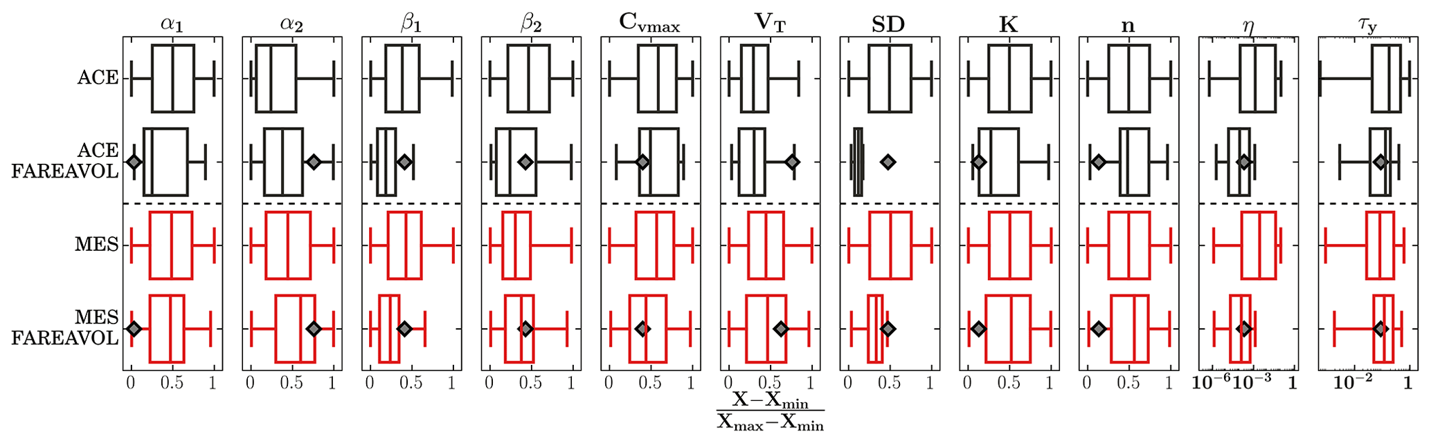
Figure 6 Effects of applying a flood area–volume observational constraint (FAREAVOL) on parameter identifiability. Results are displayed for Acerillas (black) and La Mesilla (red) creeks. The vertical bold line in the boxplots is the median; the body of each boxplot shows the interquartile range (Q₇₅–Q₂₅); and the whiskers represent the sample minima and sample maxima. The grey–black diamonds represent parameter values for the reference simulations.

The reference SD value is close to the upper range in La Mesilla after applying the FAREAVOL constraint, and also much larger than the resulting maximum values filtered at Acerillas. This result is somewhat expected, since SD does not provide large model sensitivities in that domain. Similarly, the reference β₁ value is within the upper range of filtered values (>Q₇₅). However, filtered η values around the baseline model parameter result from the compensation of low values of α₁ (near the minimum in the filtered range) and $C_{{\mathrm{v}}_{\max }}$ (below the median of filtered values). A similar effect is observed for τ_y, whose filtered range results from the compensation of α₂, β₂ and $C_{{\mathrm{v}}_{\max }}$. In summary, different combinations of α_1,2, β_1,2 and C_v can generate viscosity and yield stress values that are suitable to reproduce the 2015 debris flow events in Acerillas and La Mesilla. This is a well-known problem in environmental models – referred to as the equifinality, nonuniqueness or nonidentifiability of model parameters – that has been widely discussed for more than 3 decades in the hydrology literature (e.g., Beven, 2006; Kelleher et al., 2015) but not carefully addressed in the debris flow modeling community.

Figure 6 also shows different behavior in other parameters. For example, the reference values for K and n are in the lower range of the filtered ensembles, while the reference Vol _T is in the upper body of the boxplot. Low K values produce low $S_{{\mathrm{f}}_{\mathrm{2}}}$, the second term at the right hand of Eq. (3), representing viscous stress. This could be compensated for using larger values of SD, as in the reference model. These results demonstrate that equifinality in FLO-2D does not only involve rheological parameters and that SD could be an important parameter to correct the unrealistic model representation of rheology (D'Agostino and Tecca, 2006).

The main goal of this study was to characterize the sensitivity of model responses to variations in uncertain rheological parameters, using only independent information on parameter values (i.e., the situation comparable to Sobol, as proposed by Rakovec et al., 2014). Hence, the only verification dataset available (flood area and sediment volume from the March 2015 event) was used to examine the identifiability of model parameters. However, the relative importance of additional observations could be assessed through the Observation-Prediction (OPR) statistic (Tiedeman and Hsieh, 2004), and the potential new information provided by field data (e.g., sedimentological and morphological characteristics) for a specific parameter (e.g., α₁ and β₁) could be quantified with the Parameter-Prediction (PPR) statistic (Tonkin et al., 2007). It should be noted that, in both cases, the equation for the total local variance (Eq. 7) would be different, as additional information should be incorporated (see Appendix A in Rakovec et al., 2014).

5 Summary and conclusions

We performed a sensitivity analysis on the parameters of a widely used numerical debris flow model (FLO-2D) and assessed the effects of applying observational constraints on parameter identifiability. Our study domains are two morphologically different ravines, Acerillas and La Mesilla, located in the Atacama region (∼29^∘ S, 70^∘ W), Chile. While Acerillas is characterized by a straight and well-defined channel with almost non-alluvial fans, La Mesilla has a big alluvial fan where deposition is prone to occur.

We found that β₁ – a parameter used to estimate the fluid mixture viscosity – provides the largest sensitivities in the variables analyzed, followed by SD – a model parameter used to represent flow detention. Interestingly, the relative importance of β₁ and SD depends on the study site, with the former being more important for Acerillas and the latter being more important for La Mesilla. These results suggest that, while rheological processes dominate flow behavior at Acerillas (straight channel with small alluvial fan), sedimentation and detention processes control flow in La Mesilla (big alluvial fan). Although the total mobilized sediment Vol_T does not have an effect on Vol_dep, it is important for representing flow velocity, as Vol_T is used to estimate C_v(t), a key parameter for fluid rheology. Finally, model results seem to be almost insensitive to Manning's roughness coefficient n, while DELSA sensitivities for the remaining parameters are of second-order importance and provide similar indices.

The comparison between the original model parameter ranges (N=500) and the ensemble resulting from applying observational restrictions shows that SD and β₁ (i.e., η) are the parameters whose identifiability is mostly improved, while others practically preserve their original range. In addition, we obtain that different combinations of model parameters (including those that describe rheology) can provide very similar results, indicating that equifinality is present in FLO-2D. Our results also support the idea that single-phase rheological models lack a strong physical basis (Iverson, 2003), and, therefore, their determination requires expert knowledge. However, an encouraging finding is that the final deposited volume Vol_dep and maximum flood area A_max contain considerable information for identifying model parameters.

We obtain that SD strongly affects model results at La Mesilla, having also large effects on simulated deposited volumes at Acerillas. Moreover, this study provides evidence that SD is one of the most important parameters controlling flow behavior and could possibly surrogate rheology in the model (D'Agostino and Tecca, 2006). One-phase debris flow models still lack robust representations of complex process interactions during flow stopping that produce temporal and spatial changes in fluid rheology. Thus, these rheological changes have been replaced by simpler approaches (e.g., the incorporation of SD).

Future investigations should aim to improve the structure of debris flow models and hence achieve better simulations of deposition and erosion processes, stopping phases, and changing rheologies. Further, the development of computationally frugal methods to improve the understanding of parameter interactions in environmental models emerges as an attractive avenue for future research.