the Creative Commons Attribution 4.0 License.
the Creative Commons Attribution 4.0 License.
 | 19 Jun 2020
Snow avalanche detection and mapping in multitemporal and multiorbital radar images from TerraSAR-X and Sentinel-1
Raphael Wicki
Sämi Holenstein
Simone Baffelli
Yves Bühler
Snow avalanches can endanger people and infrastructure, especially in densely populated mountainous regions. In Switzerland, the public is informed by an avalanche bulletin issued twice a day during winter which is based on weather information and snow and avalanche reports from a network of observers. During bad weather, however, information about avalanches that have occurred can be scarce or even be missing completely. To assess the potential of weather-independent radar satellites, we compared manual and automatic change detection avalanche mapping results from high-resolution TerraSAR-X (TSX) stripmap images and medium-resolution Sentinel-1 (S1) interferometric wide-swath images for a study site in central Switzerland. The TSX results were also compared to available mapping results from high-resolution SPOT-6 optical satellite images. We found that avalanche outlines from TSX and S1 agree well with each other. Cutoff thresholds of mapped avalanche areas were found with 500 m2 for TSX and 2000 m2 for S1. S1 provides a much higher spatial and temporal coverage and allows for mapping of the entire Alps at least every 6 d with freely available acquisitions. With costly SPOT-6 images the Alps can even be covered in a single day at meter resolution, at least for clear-sky conditions. For the SPOT-6 and TSX mapping results, we found a fair agreement, but the temporal information from radar change detection allows for a better separation of overlapping avalanches. Still, the total mapped avalanche area differed by at least a factor of 3 because with radar mainly the avalanche deposition zone was detected, whereas the release zone was very visible already in SPOT-6 data. With automatic avalanche mapping we detected around 70 % of manually mapped new avalanches, at least when the number of old avalanches is low. To further improve the radar mapping capabilities, we combined S1 images from multiple orbits and polarizations and obtained a notable enhancement of resolution and speckle reduction such that the obtained mapping results are almost comparable to the single-orbit TSX change detection results. In a multiorbital S1 mosaic covering all of Switzerland, we manually counted 7361 new avalanches which occurred during an extreme avalanche period around 4 January 2018.
- Article
(11027 KB) - Full-text XML
- BibTeX
- EndNote


Snow avalanches frequently threaten people and infrastructure in Switzerland and other mountainous countries. Every winter, dozens of people caught in avalanches suffer serious injuries or even die (Techel et al., 2016), and roads and railways have to be closed during periods of high avalanche danger. To inform about the current avalanche danger levels, ranging from 1 (low) to 5 (very high) on the European Avalanche Hazard Scale (Meister, 1995), the WSL Institute for Snow and Avalanche Research (SLF) publishes an avalanche bulletin twice a day during winter (SLF, 2018e). The bulletin is written by avalanche experts who analyze weather station data, local snow conditions, detailed weather forecast information, and avalanche occurrence reported by a network of in situ observers. Unfortunately, during high avalanche activity, low visibility and closed valleys and ski resorts can lead to incomplete or missing avalanche occurrence information. In such situations, as happened in Switzerland in January 2018 and 2019, avalanches can be mapped manually in optical airborne images (Bühler et al., 2009; Eckerstorfer et al., 2016; Korzeniowska et al., 2017) or satellite images which have to be tasked in rapid mapping mode (Scott, 2009; Lato et al., 2012; Bühler et al., 2019). The resulting avalanche outlines can then be used to update avalanche databases which are of great value for hazard mapping and mitigation measure planning (Rudolf-Miklau et al., 2014). As manual mapping is very time-consuming, attempts have been made to automatize avalanche mapping in optical data (Bühler et al., 2009; Lato et al., 2012; Frauenfelder et al., 2015; Korzeniowska et al., 2017). To provide weather-independent observations, the Alpine Avalanche Forecast (AAF) service evaluated terrestrial and spaceborne radar images (Bühler et al., 2014). They concluded that medium to large avalanche events could be mapped using very-high-resolution radar satellites but with the drawbacks of limited availability and high costs. Nevertheless, for freely available but medium-resolution Sentinel-1 radar images few but promising manual and automatic avalanche mapping studies exist (Vickers et al., 2016; Eckerstorfer et al., 2017; Wesselink et al., 2017; Abermann et al., 2019; Eckerstorfer et al., 2019).
To evaluate the applicability of high and medium resolution radar images for avalanche detection in the Swiss Alps, we compare 10 m resolution Sentinel-1 radar images, 3 m resolution TerraSAR-X radar images, and 1.5 m resolution SPOT-6 optical images and analyze different methods using multitemporal and multiorbital radar images for two extreme avalanche events which occurred in Switzerland in January 2018.
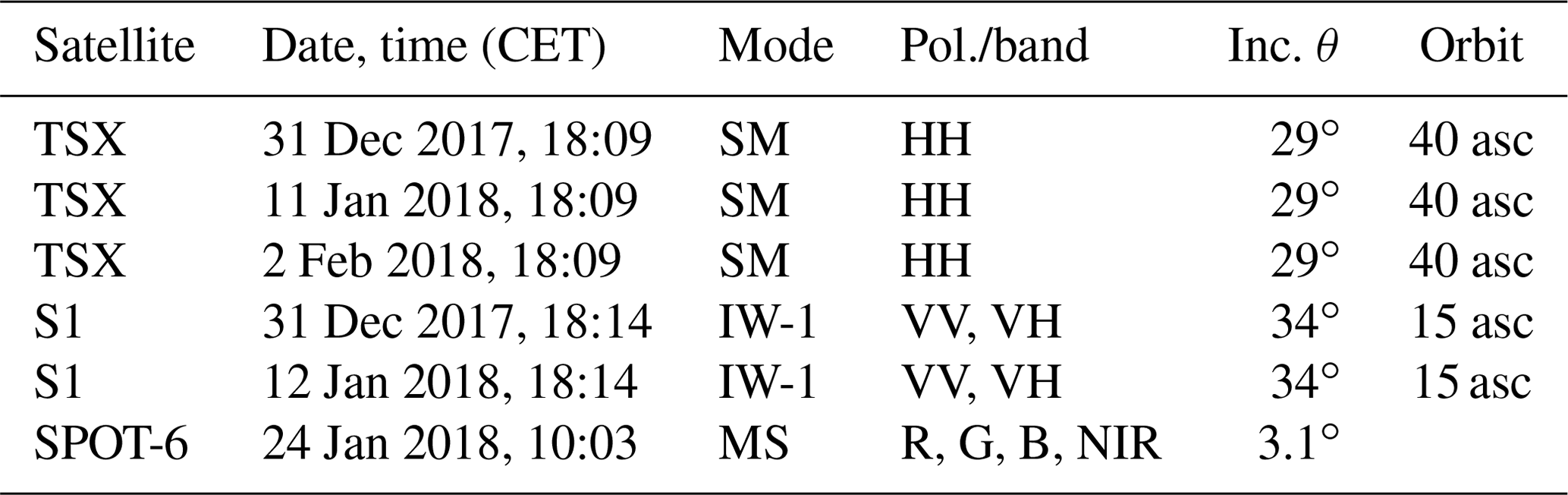
The study area (Fig. 1) was determined by the spatial and temporal availability of high-resolution radar images from the satellite TerraSAR-X (TSX), operated by the German Aerospace Center (DLR). A systematic TSX coverage is not available over Switzerland because data are acquired upon request (Werninghaus and Buckreuss, 2010). The availability of archive images, covering the two extreme avalanche events around 4 and 22 January 2018 (Fig. 2) with identical orbits, limited the study area to the Alps of Uri in central Switzerland. Acquisition dates (Table 1) were defined by the orbit repeat time, which resulted in a revisit time of 11 d for the first event and 22 d for the second one (one acquisition missing). TSX images were acquired in the X-band (9.6 GHz) with the standard stripmap mode (SM) at a nominal single-look complex (SLC) resolution of 2.3×3.3 m (rg × az). Snow and weather conditions during the two avalanche events are summarized by Bühler et al. (2019). Details are provided by Winkler et al. (2019) and SLF (2018a, b, c, d) (in German).
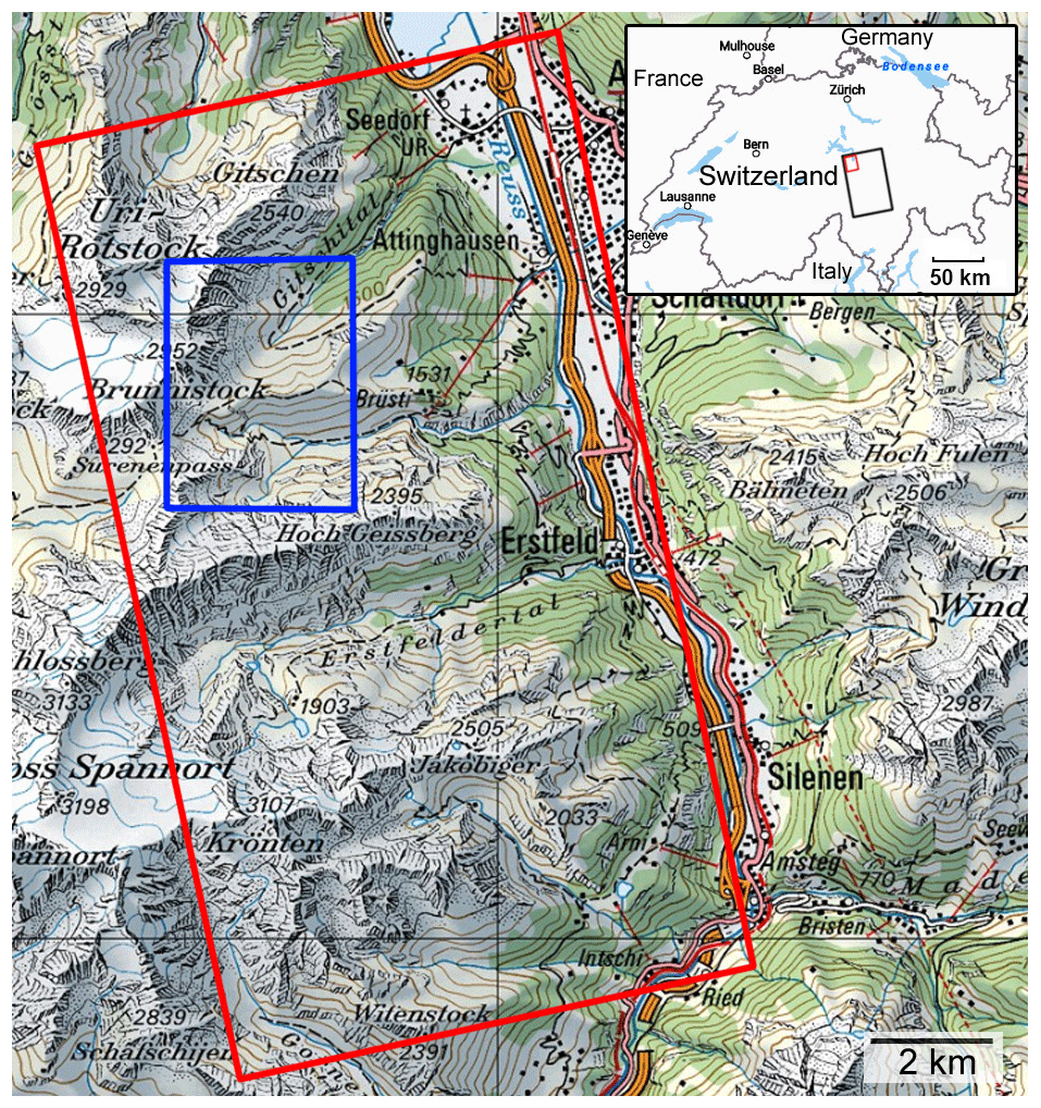
Figure 1Red rectangle: area selected for avalanche mapping. Blue rectangle: subset used to visualize radar images and mapping results (46∘51′ N, 8∘34′ E). Black rectangle in insets: full footprint of the TSX scene over Switzerland. © 2019 swisstopo (JD100042), reproduced with the authorization of swisstopo (JA100120).
Table 1Satellite images with local acquisition time (CET is UTC+1). Acquisition modes are stripmap (SM), interferometric wide-swath (IW), and single-pass multi-strip (MS) collection. S1 images used for the composite of Switzerland are listed in Table A1.
The full TSX scene (black rectangle in the inset in Fig. 1) covers 55 km × 35 km, but for the analysis we selected an area of 15.3 km × 8.6 km (red rectangle in Fig. 1) where both the TSX and the validation data (Bühler et al., 2019) show a very high avalanche activity. The selected area contains steep topography which ranges from 400 to 3200 m a.s.l. For visualization of results we show in the following figures only a small subset (blue rectangle in Fig. 1) of the analyzed area.
Radar images of the satellite Sentinel-1 (S1) were analyzed for comparison. S1 images are acquired globally and systematically and are free and openly available for download within 24 h after acquisition (ESA, 2012). Currently, S1 consists of two satellites, S1-A and S1-B, which alternately image central Europe every 6 d from the same orbit with an SLC resolution of 2.7×22.5 m (rg × az) in the interferometric wide-swath mode (IW). The S1 images, covering 250 km × 170 km, were selected such that they had orbits and acquisition times similar to those of TSX (Table 1).
The first analyzed images of both satellites were acquired on 31 December 2017 a few minutes after 18:00 LT (local time) (Table 1) and before the first avalanche event on 14 January 2018 (Fig. 2). The second TSX image was acquired after the event on 11 January 2018 and the second S1 image 1 d later (12 January 2018). For the day between, Fig. 2 shows a very low avalanche activity and meteorological conditions were relatively stable (SLF, 2018b).
To assess avalanche detection for all of Switzerland, S1 acquisitions were carefully selected from multiple orbits during a 5 d period from before and after the first event (gray shading in Fig. 2, list of acquisitions in Table A1).
To analyze the second avalanche event, the SLF ordered optical SPOT-6 images acquired 1 d after the event with the single-pass multi-strip collection mode. With this mode most of the Swiss Alps (300 km × 40 km) could be imaged in a single day (24 January 2018), at a resolution of 1.5 m. These images were visually searched for avalanches by an expert (Bühler et al., 2019). For comparison we used a third TSX image from 2 February 2018, acquired 9 d later.
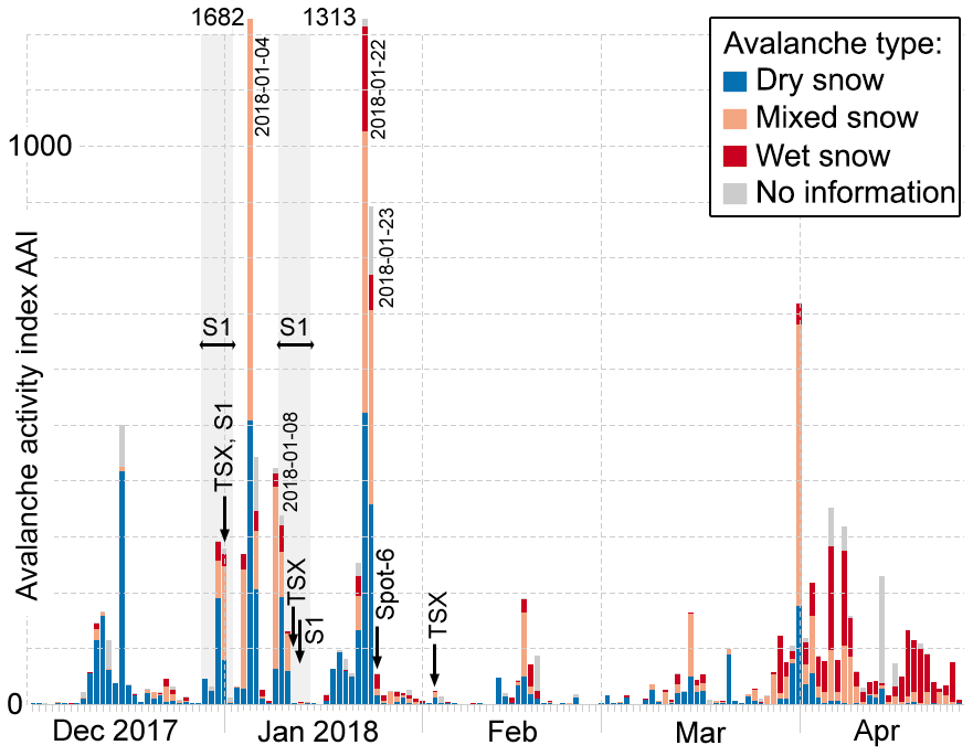
Figure 2The avalanche activity index is the weighted sum of all reported avalanches for Switzerland (Schweizer et al., 1998, 2003). Dry-snow avalanches which started high up but were slowed down at medium altitude by wet snow are indicated as “mixed snow” in the legend. Satellite acquisitions dates are indicated by arrows. Images for the multiorbital S1 composite were acquired during the gray shaded periods (see also Table A1). Figure modified after Winkler et al. (2019).
We detected avalanches based on their bright radar backscatter signal and their visual appearance (shape). Figure 3 illustrates a classification scheme from the International Commission of Snow and Ice (1981). The scheme suggests that all avalanche types are composed of three different zones but for some avalanche types (e.g., loose snow avalanches) zones can be difficult to differentiate. The most upslope zone is the release area (Fig. 3, blue) with a smooth surface caused by the failure of the weak layer, followed by the zone of transition (purple) with the stauchwall and some deposition caused by the terrain roughness, and finally the tongue-shaped zone of deposition (red) at the bottom which is covered by densely compacted snow granules.

The radar backscatter signal of the different zones depends on their snow properties. In first-order scattering physics the total backscatter intensity of a snowpack, , can be composed of scattering from the snow surface, , snow volume scattering, , scattering from the ground below the snowpack, , and scattering from higher-order interactions between different structures in the snowpack :
Currently, there exists no specific model tailored to the backscatter properties of snow avalanches (see Eckerstorfer and Malnes, 2015, Sect. 5.3); however, general scattering physics from bi-continuous media and rough surfaces can be applied. In that sense, scattering in snow increases with the spatial correlation length of ice grains (Wiesmann et al., 1998) and also with increased surface and interface roughness and with decreasing incidence angle θ (Leader, 1971; Fung and Eom, 1982; Kendra et al., 1998).
For plain dry snow of a few meters depth, scattering at the ground usually dominates the signal because microwaves between 1 and 10 GHz are weakly scattered at the snow surface and within the snow volume and therefore penetrate the snowpack to the ground (Xu et al., 2012; Cumming, 1952; Rignot et al., 2001); see also conclusion and simulations in Leinss et al. (2015). For dry snow the ground roughness determines the backscatter signal, but for smooth ground mainly forward scattering (away from the sensor) occurs. For deeper snow or higher frequencies the signal can be dominated by volume scattering (Watte and MacDonald, 1970).
In contrast to plain dry snow, snow is deeper and denser in the deposition zone where the surfaces of the avalanche debris can be very rough. Because of the higher dielectric contrast due to the higher permittivity (Matzler, 1996), the contribution of and to the total backscatter intensity increases. Both the rough surface and the debris volume should scatter radiation more omnidirectionally (diffuse scattering) compared to an undisturbed snowpack over smooth ground (more specular scattering).
For plain wet snow incoming radar waves are weakly backscattered at the air–snow interface because most radiation is lost by absorption (Tiuri et al., 1984; Cumming, 1952) and also by forward scattering as observed in Sect. 3.2 of Lucas et al. (2017) and described by the Fresnel coefficients for dielectric media. With negligible volume and ground contribution from wet-snow avalanche debris, the dominant backscatter signal must result from omnidirectional scattering at the increased surface roughness in the deposition zone of avalanches (Eckerstorfer and Malnes, 2015, Sect. 5.3).
Based on the above arguments, the zone of origin should be very difficult to detect with radar because the weakly scattering snow volume is reduced without major changes in the surface roughness. The zone of transition should be only sometimes visible, depending on the deposition of avalanche debris. Therefore, mostly the deposition zone should be visible as a brighter backscatter signal and the mostly elongated, tongue-shaped geometry.
To obtain a high backscatter contrast with respect to the avalanche surroundings, the local incidence angle θ should be far away from zero (i.e., away from layover) to avoid the intense specular back-reflection from smooth surfaces. Therefore, the visibility of avalanches in radar images should be much better for slopes facing off the radar. These slopes are also imaged with a higher ground-range resolution δsr∕cos θ which can be close to the full slant-range resolution δsr.
4.1 Data preprocessing
All radar products were downloaded in the SLC format. The data were preprocessed with the ESA SNAP Sentinel-1 toolbox and also with the GAMMA software for comparison. The workflow using GAMMA was implemented with Nextflow (Di Tommaso et al., 2017) to speed up execution and code development and to ensure a reproducible analysis. Preprocessing consists of coregistration, multilooking for reduction of radar speckle (TSX: 6 px × 5 px, S1: 4 px × 1 px), orthorectification, and generation of radar shadow and layover masks. The SNAP workflow for S1 images is shown in Fig. A1. We did not apply any radiometric terrain correction as the visible topography helps to identify the avalanche path direction.
For orthorectification we used the Swiss elevation model SwissAlti3D (2013) downsampled from 2 to 30 m resolution. We noticed, however, that despite using the same DEM and output resolution, sharp topographic features seem to be better orthorectified with the GAMMA software, which might use a more precise spatial interpolation. The radar images were orthorectified to a resolution of 5 m × 5 m (TSX) and 15 m × 15 m (S1), and the backscatter signal in decibels was saved to GeoTIFF files. The exact radiometric normalization is irrelevant, because we did not apply any radiometric terrain correction (Small, 2011), and different ellipsoidal corrections (, ) differ only by almost constant factors. Since the TSX data were acquired with a single polarization (the co-polar channel HH), we also used only the co-polar channel (VV) of the two available polarizations of S1 to obtain a fair comparison. For the multiorbital composites, we used both polarizations of S1 (VV, VH).

Figure 4Subsets of the change detection images of the study area from (a) TSX and (b) S1, acquired with ascending orbits (view from left to right) and incidence angles of 29 and 34∘. Arrows in (a) indicate old avalanches overrun by new ones. (c) S1 multiorbital composite (28 December 2017–1 January 2018 vs. 9–12 January 2018) with (d) nonlocal mean filter applied. All TerraSAR-X and Copernicus Sentinel data (2019) were orthorectified with the swissALTI3D © 2019 swisstopo (JD100042), reproduced with the authorization of swisstopo (JA100120).
4.2 Two-image composite avalanche detection
Although avalanches could be manually detected in single radar images they are difficult to analyze with automatic methods. As radar systems carry their own illumination system, the backscatter signal is primarily determined by topography and land cover type. It is therefore common practice to analyze change detection images to separate sudden backscatter changes from stable topographic and land cover features (Wiesmann et al., 2001; Eckerstorfer and Malnes, 2015). To correct for large-scale backscatter changes due to wet snow, a 500 m high-pass filter was applied to the backscatter difference between two consecutive images. Examples for TSX and S1 are shown in Fig. 4a and b. To create the images, the backscatter intensities in decibels were normalized by clipping the lower and upper 1 %. Consecutive images were then stored in the channels [R, G, B] = [img2, img1, img1] so that backscatter changes are visible by the red–cyan contrast in the RGB images. From these images (TSX and S1) avalanche outlines were drawn manually.
Such colored change detection images allow for a temporal classification of avalanches into three classes (new, old, unsure). New avalanches appear red because of increased backscattering and are therefore assumed to have occurred between the first and the second acquisitions. Old avalanches, with a decreasing backscatter signal, appear blue and are therefore assumed to have occurred before the first acquisition. Bright features with unchanged backscatter intensity appear almost white and are classified as unsure if they look like avalanches.
4.3 Multiorbital composite image for Switzerland
The free and systematic availability of S1 radar images and the short revisit period of 6 d allow for creation of an RGB composite change detection image covering all of Switzerland. Therefore, 12 images, acquired between 28 December 2017 and 1 January 2018 from different orbits, were combined into an image before the first avalanche event (4 January). Another 12 images, acquired between 9 and 12 January 2018 with an identical imaging geometry, were used for the post-avalanche event image. All images are listed in Table A1 and were preprocessed according to Sect. 4.1. To reduce radar speckle, we averaged both polarizations and weighted the cross-pol channel (VH) by the ratio of the co- and cross-pol backscatter intensities averaged over the entire scene:
Then, the weighted mean S was converted to decibels, and scenes from different ascending and descending orbits were averaged. Thereby, a relatively homogeneous bright image is obtained where layover areas lighten up the relatively dark slopes facing away from the radar without screening too many of the contained details (Fig. 4c). To further reduce noise but to preserve edges in the mosaic images, we applied a nonlocal mean filter (Jin et al., 2011; Condat, 2010). The filtered image is shown in Fig. 4d.
4.4 Relative brightness of snow avalanches
To analyze the brightness of avalanches relative to their surroundings, we calculated the ratio of the mean backscatter signal of an avalanche area and its surrounding area. Therefore, a manually generated avalanche mask was dilated once by 9 and once by 18 pixels. The difference of the two masks defines the surrounding. For the avalanche mask, the visual avalanche mask was eroded by 3 pixels to reduce manual contouring errors. To obtain statistically significant results, we calculated the backscatter ratios only for avalanches and surrounding areas larger than 100 pixels.
4.5 Automated avalanche detection
As manual avalanche mapping is time-consuming, a reliable automation of this process would make the mapping data quickly available for further application. Therefore, different methods have been developed to automatically detect avalanches mainly on the two satellite platforms S1 (Vickers et al., 2016; Wesselink et al., 2017; Abermann et al., 2019; Eckerstorfer et al., 2019) and Radarsat-2 (Hamar et al., 2016; Wesselink et al., 2017). The general workflow in these papers is quite similar to ours. All methods are based on two-image change detection, application of various masks (layover, shadow, water bodies, forest), thresholding, and filtering of extracted avalanche properties.
In addition to a shadow and layover mask, we applied a slope-dependent mask to limit the detection to potential avalanche deposition zones for which we expect the strongest backscatter change. By definition, friction is larger in the deposition zone than the downhill-slope force. Therefore, slopes steeper than 35∘, which typically occur in the zone of origin, are masked out (Bühler et al., 2009).
For noise reduction but to preserve avalanche edges, a 5 px × 5 px median filter was applied to the backscatter difference images in decibels. As avalanches should have a well-defined edge, an edge mask was generated by applying a Sobel filter with a 5×5 kernel to the median filtered difference image.
In the median filtered difference image, from all pixels brighter than a threshold of 4 dB, the brightest 5 % were considered the mask of potential avalanches. The threshold was determined empirically based on TSX data, but other authors also used thresholds of 4–6 dB (Eckerstorfer et al., 2019; Karbou et al., 2018; Vickers et al., 2016). To remove isolated bright pixels from the mask, we determined around each continuous area an ellipse and removed areas with a major axis shorter than 75 m (for both TSX and S1). Additionally, only potential avalanches for which more than 10 pixels intersect with the edge mask were considered for the final avalanche mask.
4.6 Comparison between mapping results
None of the mapping results obtained from TSX, S1, or SPOT-6 can be considered to be real ground truth, and different avalanches or avalanche shapes were detected with the different methods and satellites. Also, ambiguous relations can exist when a single large avalanche in one mapping result appears as multiple smaller avalanches in another mapping result. This makes the evaluation of binary classifiers (e.g., probability of detection or false discovery rate) difficult or even impossible. We refrained from using a pixel-to-pixel comparison which would have demanded a manual mapping precision on the pixel level which contradicts the subjective mapping by an expert who sometimes estimates an avalanche outline from discontinuous avalanche patches.
As a remedy we compare results from two data sets, A and B, by reciprocal counting of avalanches which overlap in both data sets (considered “found”) and avalanches which do not overlap (considered “not found”). These numbers differ depending on the direction in which the comparison is done (A → B or B → A). Depending which data sets are considered ground truth, avalanches which were not found can be regarded either as false negative alarms (missed) or as false positive alarms (false alarm).
All numbers in this section are obtained from the study area outlined by the red polygon in Fig. 1; figures show only a subset. The full extent is shown in the Appendix, Figs. A2, A3. For conciseness we abbreviate RGB change detection images by acquisition month and day (mm-dd∕mm-dd).
5.1 TSX change detection
In the change detection image tsx(12-31∕01-11), covering the first avalanche period, a total of 267 avalanches were manually detected (Fig. A2). As detailed in Table 2, 164 avalanches were classified as new and 19 were classified as old avalanches. For 84 avalanches a clear assignment to new or old was not possible. Therefore, we assigned them to the class unsure. For example, in the upper part of Fig. 4a arrows indicate two large new avalanches which completely overrun two small old avalanches. Hence, their backscatter signal did not change and they were classified as unsure (though they could be classified as old by context information).
Table 2Number and classification of manually detected avalanches in TSX images covering the first and the second avalanche periods.

In the change detection image tsx(01-11∕02-02), covering the second avalanche period, a total of 351 avalanches were detected, composed of 170 new avalanches, 35 old ones, and 146 unsure cases. Most of these unsure avalanches were actually classified as new after the first avalanche period but overrun by new avalanches during the second avalanche period (compare Figs. A2 and A3). Therefore, the number of old avalanches seems to remain low.
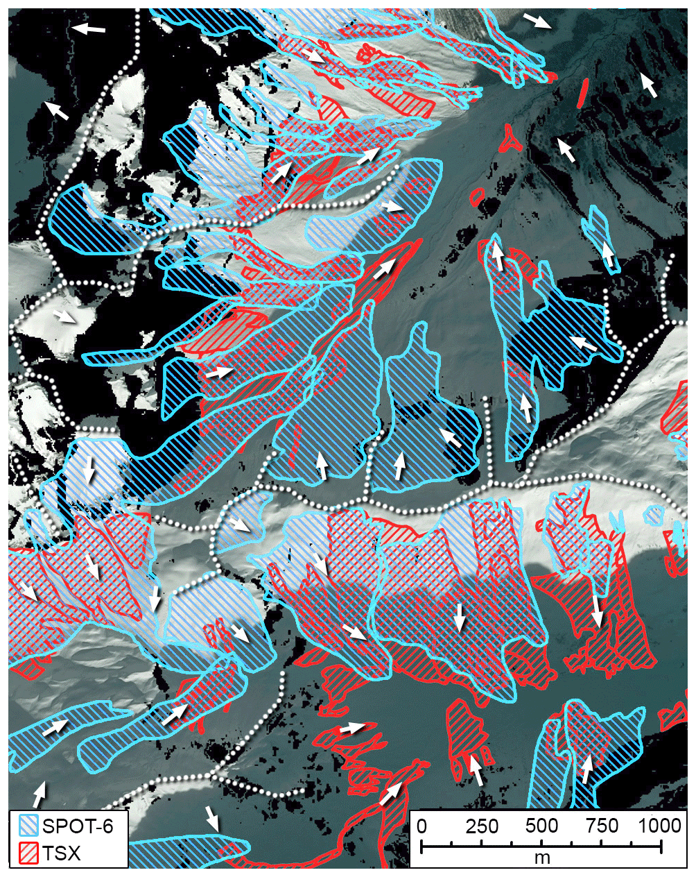
Figure 5SPOT-6/TSX: manually mapped avalanches (blue) from the SPOT-6 image on 24 January 2018 (background) vs. change detection results from tsx(01-11∕02-02) (red, all classes) in a subset of the entire study area (see Fig. 1). Radar shadow and layover are masked in black. Dots indicate mountain ridges and arrows the downslope direction. The SPOT-6 image was orthorectified with the swissALTI3D © 2019 swisstopo (JD100042), reproduced with the authorization of swisstopo (JA100120).
5.2 TSX compared to optical SPOT-6
The SPOT-6 images were acquired immediately after the second avalanche event in the morning of 24 January. Avalanches were mapped by E. Hafner in SPOT-6 images (Bühler et al., 2019). They found that only 24 % of outlines were clearly visible; 76 % of the avalanche outlines were estimated between partially visible release and deposit areas. In the study area, the SPOT-6 avalanches did not contain any age information, but the authors conclude that 20 %–45 % of avalanches were already released before the second avalanche event.
Limited by the 11 d revisit time of TSX, the next available image was acquired 9 d after the second event, in the evening of 2 February. Without knowledge of the SPOT-6 mapping results, avalanches were mapped independently in the image pair tsx(01-11∕02-02) by the second author of this work. The outlines differed significantly, however, most likely because different features (avalanche origin, path, deposit zone) are visible in optical and radar images. Therefore we decided for a feature-based comparison; i.e., overlapping polygons are considered detected in both data sets. Avalanches split up into discontinuous polygons were counted separately, even if all polygons overlap with one single large polygon in the other data set (see method Sect. 4.6).
Despite nonoptimal acquisition timing and mapping conditions, Table 3a shows for the change detection image tsx(01-11∕02-02) that 68 % (215 of 316) of the avalanches detected as new or unsure were also detected in the SPOT-6 image. Interestingly, of the remaining third (101 of 316) the majority (84 avalanches) were located in the cast shadow.
Vice versa, 44 % (125 of 286) of the optically detected avalanches were also found in the TSX change detection image (Table 3b), but more than half of the optically detected avalanches were not found. A total of 20 % (57 of 286) could not be found because they were located in the radar shadow or layover, and 36 % (104 of 286) had a too low backscatter contrast to be visible with radar. We did not find significant differences for the lower detection limits: for both TSX and SPOT-6 the smallest detectable avalanches had an area of 500 m2 (Sect. 5.6).
With the temporal information from radar change detection, 71 of the 125 avalanches detected with SPOT-6 but also with TSX (Table 3b) could be unambiguously classified into 27 new, 38 unsure, and 6 old avalanches. The remaining 54 avalanches could not be unambiguously classified, because they cover areas differentiated by radar into multiple different classes, whereas such a temporal classification is difficult with single SPOT6 images (Bühler et al., 2019).
Figure 5 shows a subset of the SPOT-6 images and visualizes the manually mapped avalanches. Especially in the lower part of the image, in the cast shadow, many small radar-detected avalanches (red) were not found in the optical analysis (blue). With radar, avalanches could generally not be detected in the radar shadow or layover (added with black), but also many other avalanches were missed by radar.
Table 3(a) Number of avalanches in TSX change detection image compared to avalanches which were also detected in the optical SPOT-6 data. (b) Reverse correspondence of avalanches from SPOT-6 to new and unsure avalanches detected by radar. Avalanches which were not found are grouped depending on their location in the cast shadow (a) or in the radar shadow (b).
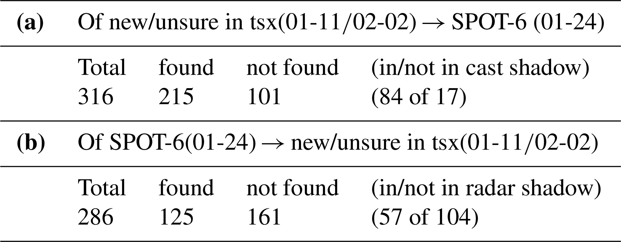
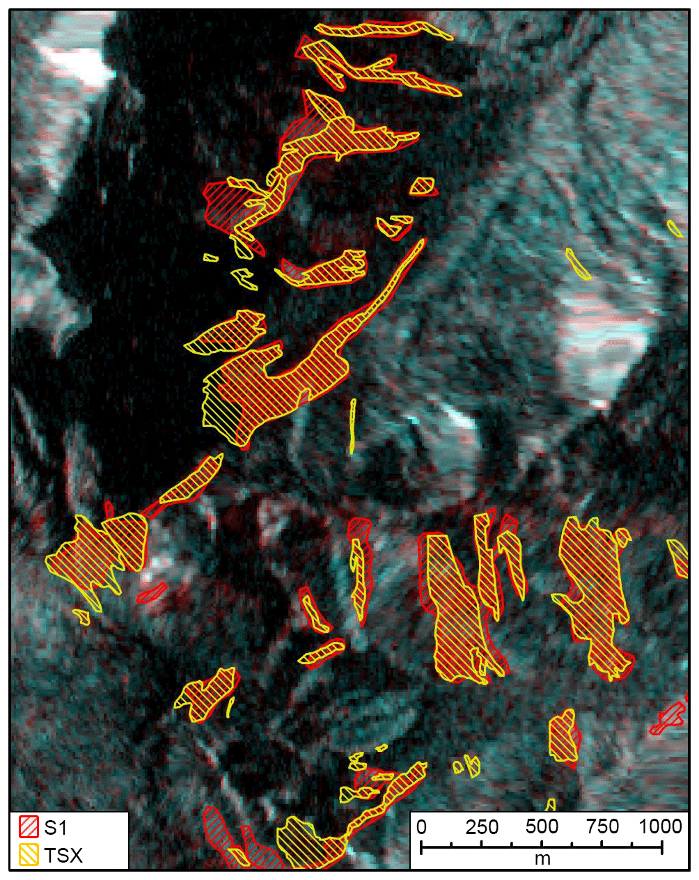
Figure 6S1/TSX: manually mapped new avalanches (in red) from the change detection image S1(12-31∕01-12) compared to manually mapped new avalanches from tsx(12-31∕01-11), in yellow. No mask is shown for avalanches classified as old or unsure. The masks were derived from the radar images shown in Fig. 4a and b. Image orthorectified with swissALTI3D © 2019 swisstopo (JD100042), reproduced with the authorization of swisstopo (JA100120).
5.3 TSX compared to S1 change detection
To assess the added value of high-resolution TSX images, we compared them to medium-resolution S1 images. We chose the first avalanche period to simplify counting because of fewer overlapping old and new avalanches. In the S1 change detection image S1(12-31∕01-12) a total of 89 new, 13 unsure, and 16 old avalanches were found. The S1 image shows a significantly lower resolution than TSX (Fig. 4a vs. Fig. 4b); therefore small avalanches are more likely to be missed.
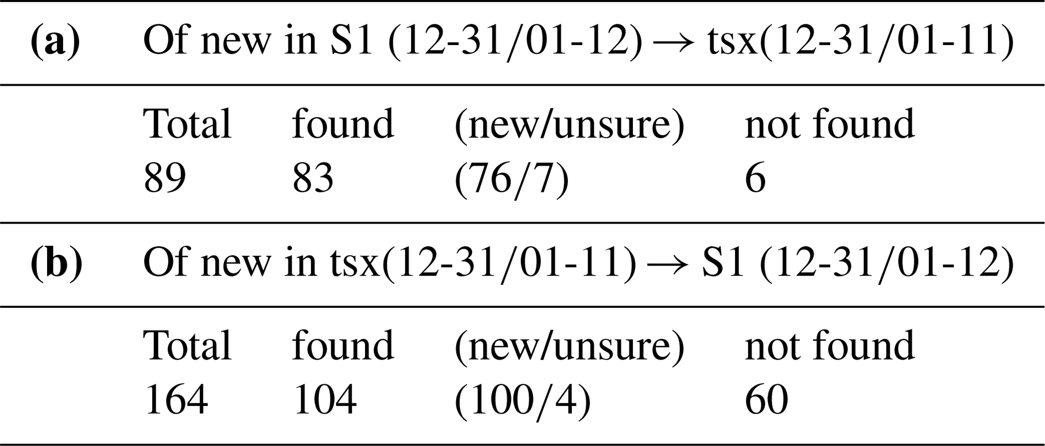
As detailed in Table 4, from the 89 new avalanches, 83 were also found by TSX. They correspond to 76 new and seven unsure avalanches; six avalanches were not found. Vice versa, two-thirds (104 of 164) of the avalanches found in tsx(12-31∕01-11) – indicated by yellow masks in Fig. 6 – correspond to the 83 avalanches also found with S1 (red mask). One-third (60 of 164) were not found, mostly because they were too small to be detected with S1. As detailed in Sect. 5.6, we found that the smallest avalanches detectable by S1 have an area of around 2000 m2.
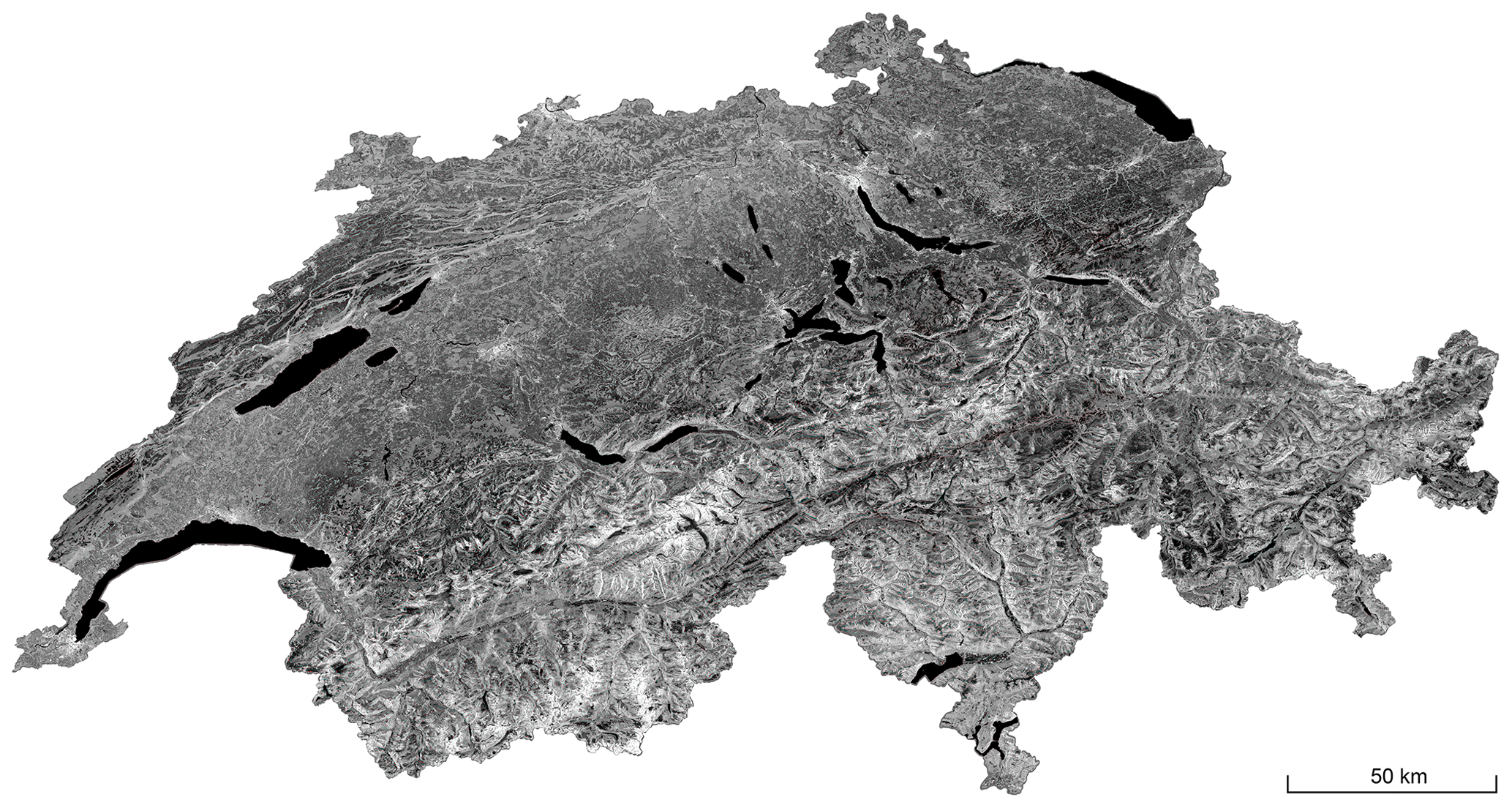
Figure 7In the 15 m resolution multiorbital S1 change detection mosaic, covering all of Switzerland for the first avalanche period around 4 January, we manually counted 7361 new avalanches. When zooming into the image, which is available online at 15 m resolution (Leinss et al., 2019), many avalanches are visible in red. The image is combined from each of the 12 acquisitions from 28 December 2017 until 1 January 2018 and from 9 to 12 January 2018. All Copernicus Sentinel scenes (2019) were orthorectified with the swissALTI3D © 2019 swisstopo (JD100042), reproduced with the authorization of swisstopo (JA100120).
Table 4(a) Number of manually detected new avalanches in S1(12-31∕01-12) which were also detected as new or unsure in the change detection image tsx(12-31∕01-11). (b) Reverse correspondence.
5.4 Multiorbital S1 change detection composite
By combining S1 acquisitions from multiple ascending and descending orbits, we minimized areas affected by radar layover (areas with radar shadow appear as layover when imaged from the opposite pass direction). A multiorbital change detection composite covering all of Switzerland during the first avalanche period is shown in Fig. 7. For noise reduction, a nonlocal mean filter was applied. In the full 15 m resolution image, which is available online (Leinss et al., 2019), we manually counted 7361 avalanches (without drawing avalanche outline polygons). We found that avalanches reaching below the wet-snow line (dark in Fig. 7) were much more visible than avalanches from the dry-snow zone (bright regions in Fig. 7). The subset shown in Fig. 4c illustrates the mitigation of layover (in the upper and lower right side of the image), the speckle reduction, and the enhanced resolution compared to the single-orbit S1 image in Fig. 4b. Only areas near radar shadow lose contrast and show a reduced avalanche visibility because the added layover image does not contain useful information.
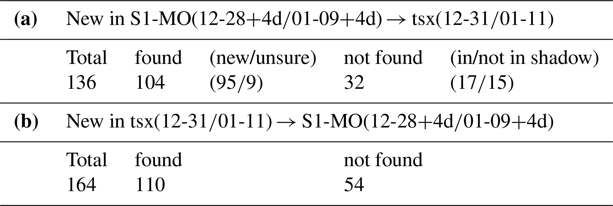
The comparison of the multiorbital S1 mapping results with the high-resolution TSX data is detailed in Table 5. In the study area a total of 136 new avalanches were manually detected in the multiorbital image (S1-MO). Of these, 104 avalanches match with avalanches detected in the corresponding single-orbit TSX change detection scene (95 of them with new avalanches, nine with unsure), whereas 32 avalanches were not found with TSX. A total of 17 of the 32 avalanches could not be detected because they are in the shadow/layover areas of TSX. Vice versa, 110 of 164 TSX avalanches were also detected in the multiorbital S1 composite whereas 54 TSX avalanches were not detected.
Table 5(a) Number of new avalanches in the S1 multiorbital change detection image (S1-MO) compared to avalanches in the TSX change detection image. Reverse correspondence in (b).
5.5 Automated avalanche detection
For the implemented automatic avalanche detection algorithm, we chose a threshold of 4 dB for the relative brightness of avalanches which corresponds to the upper 82 % of the avalanche brightness distribution shown in Fig. 8a. The figure is based on 99 of 164 new avalanches which cover more than 100 pixels (Sect. 4.4) and which were selected from tsx(12-31∕01-11) in the study area (red rectangle, Fig. 1). The threshold to mask out areas steeper than 35∘ (Sect. 4.5) is supported by the slope-dependent distribution of avalanche pixels in Fig. 8b. With these settings, the automatic methods identified about two-thirds of the manually identified avalanches in the same image pair. Here we considered the manually determined avalanche mask as a proxy for the true extent of the deposition zone. We are aware that the significance of such a comparison is limited. Nevertheless, the advantage of this comparison is that the performance of the detection algorithm is directly compared to the results of a human avalanche mapping expert.
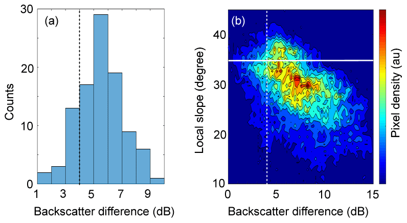
Figure 8(a) Histogram of the mean relative brightness of avalanches compared to the surrounding area for manually mapped new avalanches of tsx(12-31∕01-11) in the study area (red polygon, Fig. 1). (b) Relative brightness of the avalanche pixels in relation to the local slope angle. Lines indicate the thresholds for the backscatter difference (dashed) and the slope-dependent mask (solid).
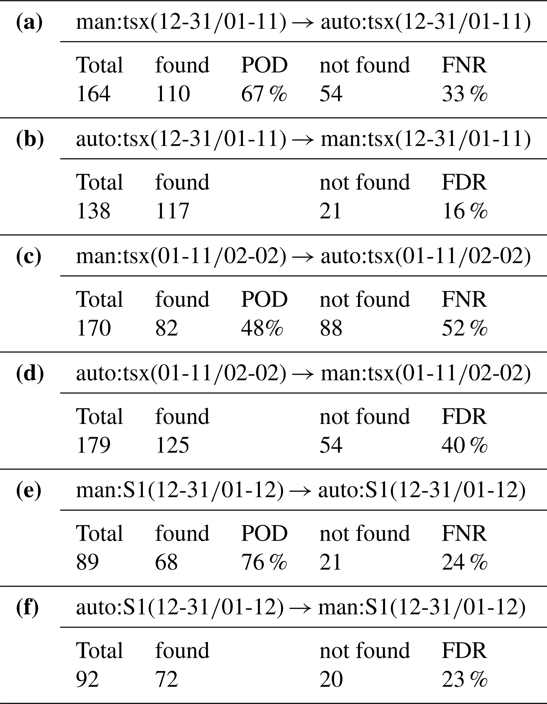
For the first image pair tsx(12-31∕01-11) Table 6a details that 110 of 164 manually mapped new avalanches were also found with the automated detection whereas 54 were not found. As shown in Fig. 9, these “missed” avalanches are often small avalanches which were filtered out by the algorithm. Vice versa, of 138 automatically detected avalanches 21 were not found manually (Table 6b).
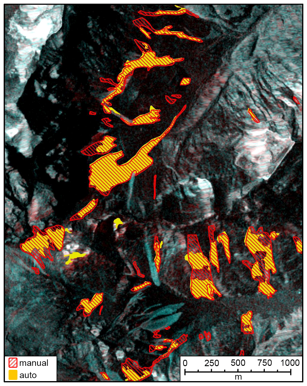
Figure 9TSX: comparison of manually mapped new avalanches (red) with automatic mapping (yellow) for the acquisition pair tsx(12-31∕01-11). Figure 4a shows the pair without a mask. Image orthorectified with the swissALTI3D © 2019 swisstopo (JD100042), reproduced with the authorization of swisstopo (JA100120).
When considering the total number (164) of manually mapped avalanches in the study area as truth, one can assign avalanches also found automatically to true positive (TP = 110), i.e., correctly detected. The remaining avalanches, which were not automatically detected, are then assigned to false negative (FN = 54), i.e., incorrectly rejected. With this assumption the probability of detection (POD) and the miss rate or false negative rate (FNR) can be calculated:
Further, one can assign automatically detected avalanches not found manually to false positives (FP = 21), i.e., incorrectly detected. Assuming that the number of correctly detected avalanches is given by TP = 110, the false discovery rate (FDR) reads
where one obtains a POD = 67 %, a miss rate FNR = 33 %, and a false discovery rate FDR = 16 % for the first TSX pair.
For the second image pair tsx(01-11∕02-02) only 82 of 170 manually detected new avalanches were automatically found whereas 88 were not found (Table 6c). Vice versa, 54 of 179 automatically detected avalanches were not found manually (Table 6d). Assuming again that the manually detected avalanches are the true avalanches, one obtains a POD of 48 %, a FNR of 52 %, and a FDR = 40 %. The results are expected to be worse compared to the first period, because mapping of new avalanches was very difficult for the second period where many old and new avalanches overlapped such that many unsure cases occurred for which the backscatter signal changed less than the threshold of 4 dB.
The automated algorithm was also run on the image pair S1(12-31∕01-12). As detailed in Table 6e, 68 of 89 manually detected new avalanches were also found automatically whereas 21 were not found. Vice versa, of 92 automatically mapped avalanches 72 were also found manually and 20 were not found (Table 6f), resulting in a POD = 76 %, a FNR = 24 %, and a FDR = 23 %.
The higher POD and lower FNR for S1 compared to TSX indicate simply that, by using S1 data, the automatic method detects a larger fraction of the manually detected avalanches. It does not indicate that results obtained from S1 are better compared to TSX data where in total more avalanches were detected.
Table 6Number of automatically detected new avalanches compared to the number of manually detected new avalanches.
5.6 Size distribution of detected avalanches
The size distribution of detected avalanches depends on sensor resolution and also on which features are actually visible to the sensor. For radar sensors it is likely that only the deposit area is mapped, whereas for the SPOT-6 data set care was taken to map (or at least estimate) the entire avalanche area, including the release area (Sect. 5.2). Because with radar only partial areas were mapped, size distributions as shown in Fig. 10a may appear shifted. To provide a more detailed insight, we plotted the cumulative area of all avalanches sorted by their apparent area Ai in Fig. 10b.
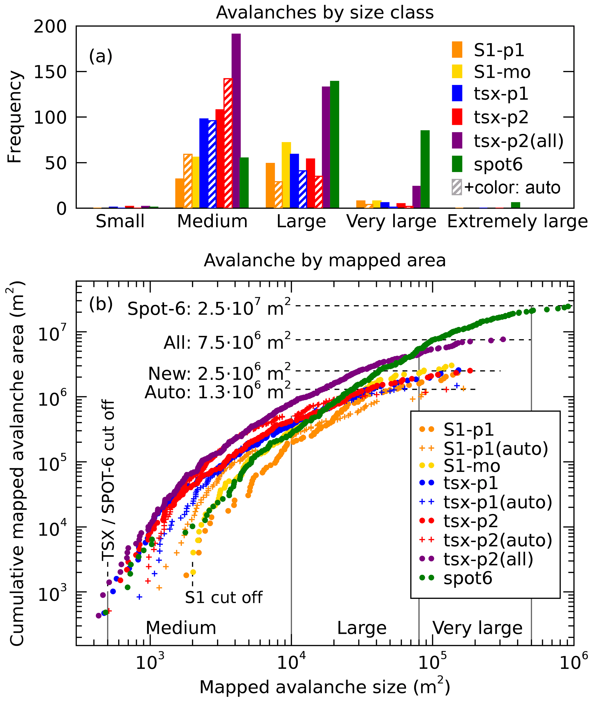
Figure 10(a) Classification of mapped avalanche area into size classes according to Bühler et al. (2019). (b) The cumulative avalanche area () plotted over avalanche size (Ai) reveals that the smallest avalanche size detected by TSX and SPOT-6 is about 500 m2, 2000 m2 for S1, and around 1000 m2 for the automatic methods. The total cumulative areas differ by an order of magnitude: with radar only bright deposit areas of new avalanches were mapped automatically (1.3×10⁶ m2), and less-bright areas were added manually (2.5×10⁶ m2). Summing all classes (new, old, unsure) in TSX images results in 7.5×10⁶ m2, which is one-third of the cumulative area of the SPOT-6 outlines (2.5×10⁷ m2).
The smallest detectable avalanche size can be found in the lower tail of the curves in Fig. 10b: for TSX and SPOT-6 the smallest avalanches have about 500 m2, 2000 m2 for S1, and around 1000 m2 for the automatic methods.
It may come as a surprise that in the study region the total avalanche area in SPOT-6 images is an order of magnitude larger (2.5×10⁷ m2, green curve in Fig. 10b) than the total area of manually detected new avalanches from TSX and S1 (red, blue, and orange dots: 2.5×10⁶ m2). A factor of 3 remains when comparing the area of all (new, old, and unsure) avalanches detected by TSX (purple in Fig. 10b) with SPOT-6, which does not contain any age classification. Considering the fact that with radar mainly the deposition zone can be mapped, the difference of a factor of 3 is reasonable.
6.1 Radar change detection images
The temporal information from radar change detection makes it possible to differentiate relatively clearly between new and old avalanches, at least for low avalanche activity where old avalanches are rarely overrun by new ones. This can be seen as a major advantage compared to optical images for which temporally dense time series are not reliably available due to weather conditions. The missing temporal information can lead to an overestimation of the avalanche area, and Bühler et al. (2019) report that deposit areas of large avalanches (>10 000 m2) remained visible for several weeks.
Nevertheless, for strong avalanche activity, the differentiation of overlapping avalanches is difficult even with radar. For example, we found a large number of unsure avalanches for the second analyzed avalanche event (Sect. 5.1) which could be identified as new avalanches from the first event. For temporal separation, fast repeat times of current radar satellites, like 6 d when combining the two S1 satellites, are a major advantage compared to other satellites (TSX: 11 d; Radarsat: 24 d). To differentiate overlapping avalanches, a recently developed age-tracking algorithm has shown promising results (Eckerstorfer et al., 2019).
6.2 Optical mapping vs. radar change detection
Regardless of the advantages of radar change detection, the effective spatial resolution of optical sensors is higher even when radar sensors provide the same nominal resolution. This is because the intrinsically coherent synthetic-aperture radar (SAR) imaging method makes radar speckle unavoidable and requires spatial or temporal averaging. In our study, the resolution of TSX and S1 was not good enough to recognize flow structures on the avalanche surface which were well visible in the optical SPOT-6 images (Bühler et al., 2019).
Nevertheless, using TSX change detection we have mapped a similar number of avalanches (316) in the study area compared to the results from optical SPOT-6 images (286 avalanches). However, the mapped avalanche outlines differ significantly, and the outlines are sometimes split up into noncontiguous sub-polygons. This results in the fact that only 68 % of the radar-detected avalanches overlap with avalanches found with the optical data, and inversely only 44 % of optically detected avalanches were also found by radar. The fact that a larger fraction (68 % vs. 44 %) of radar-detected avalanches match with optically detected ones results from the better differentiation of adjacent avalanches into multiple classes (new, old, unsure) which were often mapped as one large avalanche with optical data. Inversely, a large number (104) of optically detected avalanches could just not be detected by radar (Table 3). When multitemporal optical data are available, a temporal differentiation is possible (Bühler et al., 2019), which, however, was done for a different region than our analyzed area.
From the analysis of avalanches detected by radar but not by optical SPOT-6 images, we found that over 80 % of these avalanches were located in the cast shadow. Similarly, in radar images no (or very poor) information is available in radar shadow and layover. However, only 35 % of avalanches not found in the radar images (but in optical images) are located in the radar shadow or layover. We think it is an important result that not only radar acquisitions are affected by (radar) shadow but that avalanche mapping using optical data also seem to be hampered by the cast shadow from tall mountains.
A main difference between SPOT-6 and radar mapping results is that the total avalanche area differed at least by a factor of 3 (Fig. 10b). We attribute this difference to the fact that with SPOT-6 avalanches were mapped more completely (origin, path, deposition zone) than with radar (mainly deposition zone). This has important consequences when comparing avalanches by pixel area rather than by overlap.
Due to unfortunate acquisition timing, the direct comparison of SPOT-6 and TSX data is not ideal: the SPOT-6 images (24 January 2018) were acquired just between the two TSX images (11 January, 2 February 2018), which left 9 d when additional avalanches could have occurred, considering about 20 cm of fresh snow on 1 February. Nevertheless, Fig. 2 indicates that the biggest number of avalanches occurred before the SPOT-6 acquisition and only about 5 % of avalanches occurred until 2 February. We confirm this by analyzing a multiorbital S1 change detection image S1(01-24+01-28∕01-30+02-03) where we did not find any new avalanches in the study area. During the elapsed 9 d surface melt also occurred, which likely has decreased the backscatter contrast between avalanches and the surrounding snow due to rounding of the snow surface. The decreased contrast could explain why 104 of 286 optically detected avalanches could not be found with TSX.
6.3 TSX compared to S1 change detection
The comparison of TSX and S1 change detection images, both of them acquired for the first avalanche period with almost identical orbits and acquisition times, shows that the S1 satellites are a valuable data source for avalanche mapping. The smallest detectable avalanches for TSX were found to be “medium” avalanches (500–10 000 m2) wider than 20 m. S1 missed many medium avalanches smaller than 2000 m2 (Fig. 10b). Similar results for S1 with a minimum cutoff of 4000 m2 were found by Eckerstorfer et al. (2019).
Still about two-thirds of avalanches detected and classified as new with TSX could also be detected with S1 (Sect. 5.3). Notably, 93 % (83 of 89) of avalanches detected by S1 could also be detected by TSX, which reflects the agreement between TSX and S1 mapping results. This is confirmed by Fig. 10b, which shows that, despite a different lower cutoff area, the total area of radar-mapped new avalanches agrees very well (2.5×10⁶ m2). Also, the shape of avalanche polygons obtained from S1 data is very similar to the shapes obtained from TSX (Fig. 6). Therefore, we consider the reduced resolution and separability of avalanches in S1 images to be much less relevant than the superior availability of S1 data.
6.4 Multiorbital composite
The combination of radar images acquired with different polarizations and from ascending and descending orbits reduced radar speckle and minimized areas affected by layover. By combining two orbits and (pairwise incoherent) polarizations, areas visible from both orbits were imaged by four independent observations. In our case of mapping all of Switzerland for a specific period, this number was even increased to six or eight observations when acquisitions with different incidence angles (from the same orbit direction) overlap. Due to the four to eight independent observations, spatial multilooking (used for speckle reduction) could be reduced to 4×1 pixels to obtain a radiometric accuracy otherwise only possible with multilooking windows of 8 … 16×2 pixels. With this multiorbital averaging method, we estimate that an effective spatial resolution of about 20 m × 20 m was achieved (TSX: about 10 m × 10 m after multilooking). This resolution enhancement can be clearly observed when comparing Fig. 4b with Fig. 4c. Also, about twice as many medium-size avalanches were detected compared to a single S1 image (Fig. 10a). However, because topography was neglected during averaging, the resolution can deteriorate in slopes facing off the radar (Sect. 3).
Another drawback of combining acquisitions from multiple dates is that no unique time stamp can be given to the “before” and “after” acquisitions. In the worst case, avalanches lose contrast if they had occurred during the collection period of the set of before images. However, in our case, we focused on the extreme avalanche event on 4 January 2018 (Fig. 2) and made sure that the before- and after-imaging periods did not overlap with the main avalanche event. For an operational use, combined (asc+desc) acquisitions must be acquired within a time period as short as possible, i.e., significantly shorter than the orbit revisit time to avoid reduced visibility by averaging out “in-between” avalanches only visible in one of the two averaged acquisitions. For S1, ascending and descending acquisitions with 1.5 to 2.5 d time difference could be used. Considering a revisit time of 6 d over Europe results in a probability of 25 %–40 % that the avalanche visibility could be reduced.
In this study we simply averaged the change detection radar images and did not apply any terrain correction. We think that more advanced methods to merge radar images from multiple orbits, for example local-resolution weighting (LRW) by Small (2012), should further improve avalanche mapping results. From the comparison with optical data, we also found that avalanches can be more clearly identified in slopes facing off the radar compared to slopes which are facing towards the radar (but not yet in layover). As detailed in Sect. 3, we think that, because of the more isotropic scattering from the rough avalanche debris surface, large local radar incidence angles should be preferably used to enhance the contrast of avalanches to the surrounding snow. Therefore, slopes facing away from the sensor should be given more weight, which is already done implicitly by LRW. Furthermore, in mountainous regions LRW already applies unequal weights for ascending and descending acquisitions, which will decrease the probability that avalanches falling in between averaged acquisitions lose their visibility.
6.5 Automated avalanche detection
For both TSX and S1 images the implemented avalanche detection algorithm performs with reasonable results, at least when the number of overlapping avalanches is low. That means that in general a few sparse events are more likely to be detected than overlapping clusters of avalanches.
Compared to the manually detected avalanches (red shading in Fig. 9), the area of automatically detected avalanches (yellow) shows a good agreement. However, the upslope parts of avalanches are often only fractionally detected because of their relatively low brightness. For a weakly visible starting or transition zone, a human observer can conclude that it must belong to the avalanche deposit situated below. Also, by choosing a threshold of 4 dB, already 18 % of the manually detected avalanches are likely to be missed (Fig. 8a). A dynamic threshold based on backscatter changes in individual image pairs could improve these results (Eckerstorfer et al., 2019). Further, minor parts of manually detected avalanches are located in slopes steeper than 35∘ (Fig. 8b), which were masked out by the automatic method.
6.6 Avalanche differentiation with different methods
The fact that no real ground truth exists makes a direct comparison of the different methods difficult. However, some methods show a much higher potential to differentiate large connected avalanche patches into multiple smaller ones than other methods. Therefore we use a reciprocal, two-way comparison of avalanche detection numbers to estimate which of the methods can better differentiate adjacent avalanches.
As a proxy for the enhanced differentiation, we define the ratio , where NA→B is the number of avalanches from data set A which were also found in data set B, and inversely NB→A is the number of avalanches in B which were also found in A. Additionally, we define the ratio NA¬B∕NA of avalanches found in A but not found in B relative to all avalanches found in A and analogue NB¬A∕NB. The meaning of the last two ratios depends on interpretation and corresponds to the false discovery rate (FDR) under the assumption that B is considered truth or alternatively to the false negative rate (FNR) if A is considered truth.
Table 7Avalanche differentiation ratios between different satellite acquisitions and methods and mutual miss and false discovery rates.
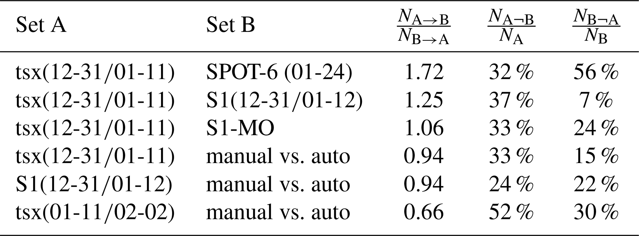
Table 7 lists the three ratios for different data sets. We interpret these numbers such that a differentiation ratio indicates that set A provides spatially more detailed results than set B. An asymmetry between the last two columns indicates that one method detects more avalanches than the other method.
From the comparison with SPOT-6, derived from Table 3, we infer that TSX change detection allows for a better differentiation of avalanches than single optical images. However, both methods show miss rates (and possibly some false detection) of 32 % and 56 % for avalanches which are not visible by the other method, which indicates a certain complementarity of optical and radar images for avalanche detection.
Compared to S1, the higher resolution of TSX allows for a 25 % better differentiation, and 37 % more avalanches were detected (derived from Table 4). Still, the false discovery rate of S1 compared to TSX is quite low (7 %).
Interestingly, the avalanche separability of the multiorbital S1 composite, including the nonlocal mean filter, is very comparable to TSX single-orbit change detection (1.06) while 33 % or 24 % of avalanches detected by one method are not visible with the other (derived from Table 5). This is because TSX detects smaller avalanches, while the multiorbital methods also detect avalanches otherwise located in slopes close to layover.
Finally, the automatic methods detect larger avalanches fairly comparably to the manual method (derived from Table 6); however, weakly visible avalanches and small avalanches which have not been automatically detected cause a miss rate of about 30 %. The apparently lower differentiation of avalanche by manual analysis results from the fact that the automatic method often detects multiple patches instead of a single avalanche which can be recognized in Fig. 9.
We studied the capabilities of the radar satellites TerraSAR-X (TSX) and Sentinel-1 (S1) to detect avalanches in two-image change detection images and multiorbital change detection composites. Manual avalanche mapping results from the high- and medium-resolution radar data (TSX, S1) and high-resolution optical data (SPOT-6) were compared to each other. An automatic detection method was developed and compared to the manual mapping results.
We conclude that both TSX and S1 radar images can provide valuable, weather-independent information about avalanche activity, even in difficult alpine terrain. Despite different lower avalanche cutoff sizes of about 500 m2 for TSX and 2000 m2 for S1, avalanche outlines and the total mapped areas agree very well between S1 and TSX.
Comparing the manual TSX and SPOT-6 mapping results, we found a reasonable agreement. The total mapped avalanche areas of TSX and S1 cover only one-third (the deposition zone) of the total mapped area (release, path, deposit) in SPOT-6 images. Interestingly, many avalanches located in the cast shadow of the SPOT-6 image were not detected, whereas they were clearly visible in a TSX image acquired 10 d later. With the automated detection algorithm we found about 60 %–80 % of the avalanches manually mapped in the same image, at least when no large number of old avalanches were present.
We found that the nonsystematic acquisition program and the possibly high cost can be considered a drawback of TSX data. Also, with the maximal swath width of 30 km in stripmap mode and a nominal revisit period of 11 d, an operational use for avalanche mapping over Switzerland is not feasible with TSX. However, the high-resolution images can provide valuable information for validation of lower-resolution mapping results for predefined test sites and if acquisitions are scheduled in advance.
Despite the lower resolution, we found that the two S1 satellites provide a convincing solution for systematic avalanche mapping because of the total swath width of 250 km and the revisit period of 6 d. Results from Norway by Eckerstorfer et al. (2018, 2019) confirm this conclusion.
With the multiorbital combination of systematically available S1 acquisitions from different orbits and with different polarizations, we minimized not only areas located in radar layover but also enhanced the radiometric accuracy and obtained a high spatial resolution of about 20 m × 20 m. In the resulting change detection image covering all of Switzerland, we manually counted in total 7361 new avalanches which occurred during an extreme avalanche period around 4 January 2018. However, we suppose that mainly avalanches reaching below the wet-snow line were detected and that likely many dry-snow avalanches were missed because of their lower contrast to the surrounding snow. A disadvantage of the multiorbital composite is the loss of precise timing of avalanches. For operational applications we therefore suggest minimizing the ratio of elapsed time between ascending and descending acquisitions and of the revisit time.
We think that avalanche mapping can be further improved with more advanced methods to combine different orbits, for example with local-resolution weighting, LRW (Small, 2012). With that, slopes facing off the radar are weighted more strongly, which not only enhances the resolution but should also increase the avalanche visibility. We found that avalanches are hardly visible in slopes facing towards the radar (but not yet in layover), and we think that the more omnidirectional scattering from the rough avalanche debris should dominate the scattering from the smooth surrounding snow only for slopes facing off the radar. As with LRW slopes are averaged with unequal weight the probability that avalanches occur between two averaged images is also reduced.
Although we could show that radar change detection mapping with TSX provides results comparable to optical SPOT-6 direct mapping, we note that our study focused on the exceptionally warm January 2018 with frequent surface melt but also with very intense snowfall periods. As the relative brightness of avalanches should increase with the water content and the amount of deposited snow, avalanches might be less visible during cold weather with little snowfall. Therefore, we think that an analysis of longer time series of radar-based avalanche mapping will provide insight into how snow and weather conditions affect the detection rate of radar-based methods.
Table A1List of S1 acquisitions used for the multiorbital change detection composite shown in Fig. 7.
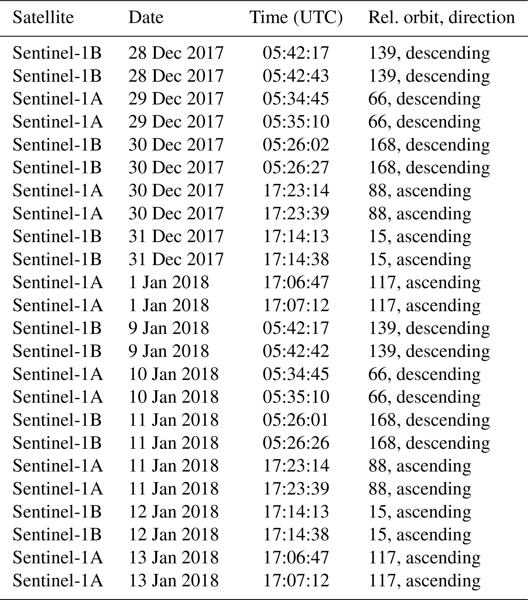

Figure A1SNAP workflow to process S1 data. The red dashed box is used for creation of the layover and shadow map.
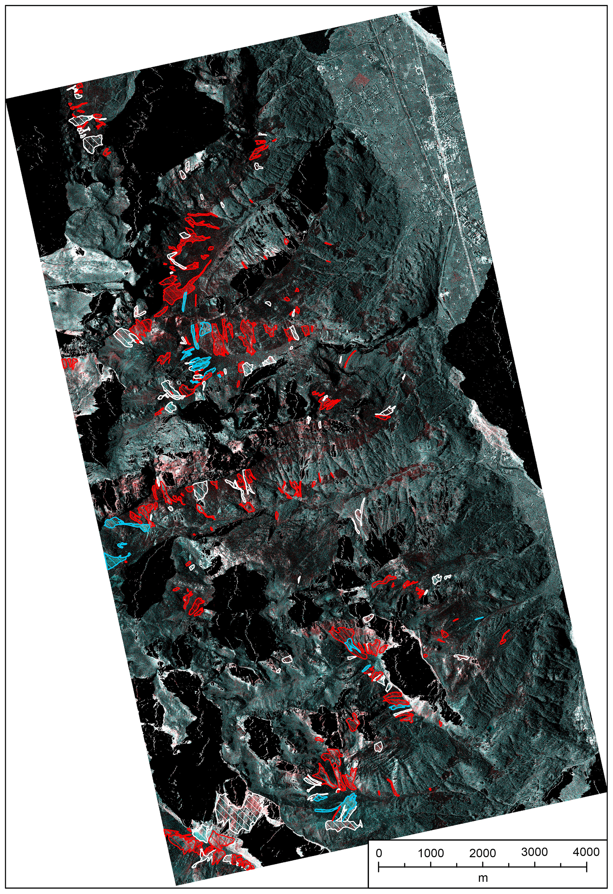
Figure A2Full extent of the RGB composite image TSX 2017-31-12 vs. 2018-01-11 with manually mapped avalanches. New avalanches are red, old avalanches are blue, and unsure avalanches are white. Areas in the radar layover and shadow are masked out (black). TerraSAR-X image orthorectified with the swissALTI3D © 2019 swisstopo (JD100042), reproduced with the authorization of swisstopo (JA100120).
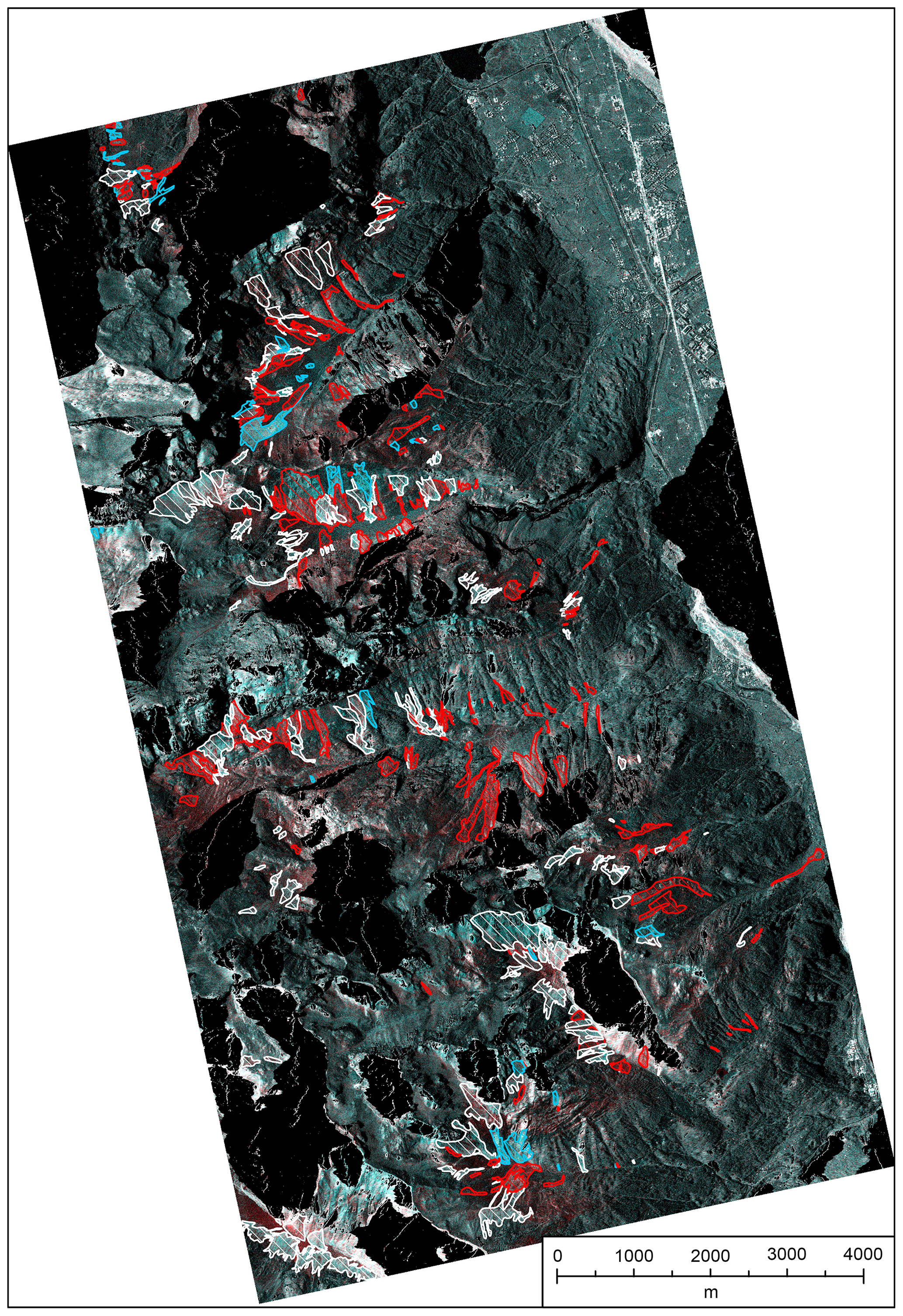
Figure A3Full extent of the RGB composite image TSX 2018-01-11 vs. 2018-02-02 with manually mapped avalanches. New avalanches are red, old avalanches are blue, and unsure avalanches are white. Areas in the radar layover and shadow are masked out (black). TerraSAR-X image orthorectified with the swissALTI3D © 2019 swisstopo (JD100042), reproduced with the authorization of swisstopo (JA100120).
TerraSAR-X data are available from the archive https://terrasar-x-archive.terrasar.com (last access: 16 June 2020) (Airbus, 2020). Copernicus Sentinel-1 data processed by ESA have been downloaded from the Copernicus Open Access Hub (https://scihub.copernicus.eu, last access: 16 June 2020) (ESA, 2020) and from the Alaska SAR Facility ASF DAAC 2018 (https://www.asf.alaska.edu, last access: 16 June 2020) (NASA, 2020). The manual mapping results from the optical data and the Sentinel-1 change detection composite of Switzerland are available online (Hafner and Bühler, 2019; Leinss et al., 2019).
SL and RW analyzed the results and wrote the manuscript together. RW did the avalanches mapping and designed the automatic detection. SL coordinated the study and implemented the nonlocal mean filter. SH, SB, and SL preprocessed the radar images. YB initiated the study and complemented the manuscript.
The authors declare that they have no conflict of interest.
We thank Elisabeth Hafner from SLF for providing the manual avalanche mask from the optical SPOT-6 data. Lanqing Huang assisted Sämi Holenstein in processing the S1 data. We are deeply grateful to Irena Hajnsek from ETH Zürich for providing the working environment, the computational resources, and her interest for this work. TerraSAR-X data are provided by the German Aerospace Center (proposal ID LAN3585). We thank Markus Eckerstorfer and the anonymous reviewer for critically reviewing the manuscript and for their helpful and constructive comments.
This paper was edited by Paolo Tarolli and reviewed by Markus Eckerstorfer and one anonymous referee.
Abermann, J., Eckerstorfer, M., Malnes, E., and Hansen, B. U.: A large wet snow avalanche cycle in West Greenland quantified using remote sensing and in situ observations, Nat. Hazards, 97, 517–534, https://doi.org/10.1007/s11069-019-03655-8, 2019. a, b
Airbus: TerraSAR-X Archive, available at: https://terrasar-x-archive.terrasar.com, last access: 16 June 2020. a
Bühler, Y., Hüni, A., Meister, R., Christen, M., and Kellenberger, T.: Automated detection and mapping of avalanche deposits using airborne optical remote sensing data, Cold Reg. Sci. Technol., 57, 99–106, https://doi.org/10.1016/j.coldregions.2009.02.007, 2009. a, b, c
Bühler, Y., Bieler, C., Pielmeier, C., Frauenfelder, R., Jaedicke, C., Schwaizer, G., Wiesmann, A., and Caduff, R.: Improved Alpine avalanche forecast service AAF, Final report, Integrated application program IAP, European Space Agency ESA, SLF, Birmensdorf, NGI, Oslo, available at: https://www.dora.lib4ri.ch/wsl/islandora/object/wsl:22266 (last access: 16 June 2020), 2014. a
Bühler, Y., Hafner, E. D., Zweifel, B., Zesiger, M., and Heisig, H.: Where are the avalanches? Rapid SPOT6 satellite data acquisition to map an extreme avalanche period over the Swiss Alps, The Cryosphere, 13, 3225–3238, https://doi.org/10.5194/tc-13-3225-2019, 2019. a, b, c, d, e, f, g, h, i, j
Condat, L.: A Simple Trick to Speed Up the Non-Local Means, working paper or preprint, available at: https://hal.archives-ouvertes.fr/hal-00512801 (last access: 16 June 2020), 2010. a
Cumming, W. A.: The Dielectric Properties of Ice and Snow at 3.2 Centimeters, J. Appl. Phys., 23, 768–773, https://doi.org/10.1063/1.1702299, 1952. a, b
Di Tommaso, P., Floden, E. W., Barja, P. P., Palumbo, E., and Notredame, C.: Nextflow enables reproducible computational workflows, Nat. Biotechnol., 35, 316–319, https://doi.org/10.1038/nbt.3820, 2017. a
Eckerstorfer, M. and Malnes, E.: Manual detection of snow avalanche debris using high-resolution Radarsat-2 SAR images, Cold Reg. Sci. Technol., 120, 205–218, https://doi.org/10.1016/j.coldregions.2015.08.016, 2015. a, b, c
Eckerstorfer, M., Bühler, Y., Frauenfelder, R., and Malnes, E.: Remote sensing of snow avalanches: Recent advances, potential, and limitations, Cold Reg. Sci. Technol., 121, 126–140, https://doi.org/10.1016/j.coldregions.2015.11.001, 2016. a
Eckerstorfer, M., Malnes, E., and Müller, K.: A complete snow avalanche activity record from a Norwegian forecasting region using Sentinel-1 satellite-radar data, Cold Reg. Sci. Technol., 144, 39–51, https://doi.org/10.1016/j.coldregions.2017.08.004, 2017. a
Eckerstorfer, M., Malnes, E., Vickers, H., Müller, K., Engeset, R., and Humstad, T.: Operational avalanche activity monitoring using radar satellites: From Norway to worldwide assistance in avalanche forecasting, in: International Snow Science Workshop, Innsbruck, Austria, 2018. a
Eckerstorfer, M., Vickers, H., Malnes, E., and Grahn, J.: Near-Real Time Automatic Snow Avalanche Activity Monitoring System Using Sentinel-1 SAR Data in Norway, Remote Sensing, 11, 2863, https://doi.org/10.3390/rs11232863, 2019. a, b, c, d, e, f, g
ESA: Sentinel-1: ESA's Radar Observatory Mission for GMES Operational Services (ESA SP-1322/1, March 2012), Tech. rep., ESA, Noordwijk, the Netherlands, 2012. a
ESA: Copernicus Open Access Hub, available at: https://scihub.copernicus.eu, last acess: 16 June 2020. a
Frauenfelder, R., Malnes, E., Solberg, R., and Müller, K.: Towards an automated snow property and avalanche mapping system (ASAM), techreport 20130092-04-R, NGI – Norwegian Geotechnical Institute, https://doi.org/10.13140/RG.2.1.1962.5446, 2015. a
Fung, A. K. and Eom, H. J.: Application of a Combined Rough Surface And Volume Scattering Theory to Sea Ice And Snow Backscatter, IEEE T. Geosci. Remote, GE-20, 528–536, https://doi.org/10.1109/TGRS.1982.350421, 1982. a
Hafner, E. and Bühler, Y.: SPOT6 Avalanche outlines 24 January 2018, https://doi.org/10.16904/envidat.77, 2019. a
Hamar, J. B., Salberg, A., and Ardelean, F.: Automatic detection and mapping of avalanches in SAR images, in: International Geoscience and Remote Sensing Symposium, 10–15 July 2016, Beijing, 689–692, https://doi.org/10.1109/IGARSS.2016.7729173, 2016. a
International Commission of Snow and Ice: Avalanche atlas: illustrated international avalanche classification, Unesco, Paris, available at: https://unesdoc.unesco.org/ark:/48223/pf0000048004 (last access: 16 June 2020), 1981. a
Jin, Q., Grama, I., and Liu, Q.: Removing Gaussian Noise by Optimization of Weights in Non-Local Means, in: 2012 Symposium on Photonics and Optoelectronics, SOPO 2012, 21–23 May 2012, Shanghai, https://doi.org/10.1109/SOPO.2012.6270436, 2011. a
Karbou, F., Coléou, C., Lefort, M., Deschatres, M., Eckert, N., Martin, R., Charvet, G., and Dufour, A.: Monitoring avalanche debris in the French mountains using SAR observations from Sentinel-1 satellites, in: Proceedings of the International Snow Science Workshop, 7–12 October 2018, Innsbruck, Austria, 344–347, 2018. a
Kendra, J. R., Sarabandi, K., and Ulaby, F. T.: Radar measurements of snow: experiment and analysis, IEEE T. Geosci. Remote, 36, 864–879, 1998. a
Korzeniowska, K., Bühler, Y., Marty, M., and Korup, O.: Regional snow-avalanche detection using object-based image analysis of near-infrared aerial imagery, Nat. Hazards Earth Syst. Sci., 17, 1823–1836, https://doi.org/10.5194/nhess-17-1823-2017, 2017. a, b
Lato, M. J., Frauenfelder, R., and Bühler, Y.: Automated detection of snow avalanche deposits: segmentation and classification of optical remote sensing imagery, Nat. Hazards Earth Syst. Sci., 12, 2893–2906, https://doi.org/10.5194/nhess-12-2893-2012, 2012. a, b
Leader, J.: The relationship between the Kirchhoff approach and small perturbation analysis in rough surface scattering theory, IEEE T. Anten. Propag., 19, 786–788, 1971. a
Leinss, S., Wiesmann, A., Lemmetyinen, J., and Hajnsek, I.: Snow water equivalent of dry snow measured by differential interferometry, IEEE J. Sel. Top. Appl. Earth Obs. Remote Sens., 8, 3773–3790, https://doi.org/10.1109/JSTARS.2015.2432031, 2015. a
Leinss, S., Holenstein, S., and Wicki, R.: Sentinel-1 change detection mosaic of Switzerland for the avalanche event of January 4th 2018, https://doi.org/10.3929/ethz-b-000376048, 2019. a, b, c
Lucas, C., Leinss, S., Bühler, Y., Marino, A., and Hajnsek, I.: Multipath Interferences in Ground-Based Radar Data: A Case Study, Remote Sensing, 9, 1260, https://doi.org/10.3390/rs9121260, 2017. a
Matzler, C.: Microwave permittivity of dry snow, IEEE T. Geosci. Remote, 34, 573–581, 1996. a
Meister, R.: Country-wide avalanche warning in Switzerland, in: Proceedings International Snow Science Workshop, Snowbird, Utah, USA, 30 October–3 November 1994, ISSW 1994 Organizing Committee, Snowbird, UT, USA, 58–71, 1995. a
NASA: Alaska SAR Facility ASF DAAC 2018, available at: https://www.asf.alaska.edu, last access: 16 June 2020. a
Rignot, E., Echelmeyer, K., and Krabill, W.: Penetration depth of interferometric synthetic-aperture radar signals in snow and ice, Geophys. Res. Lett., 28, 3501–3504, https://doi.org/10.1029/2000GL012484, 2001. a
Rudolf-Miklau, F., Sauermoser, S., Mears, A., and Boensch, M.: The Technical Avalanche Protection Handbook, Wiley, Berlin, Germany, 2014. a
Schweizer, J., Jamieson, J. B., and Skjonsberg, D.: Avalanche forecasting for transportation corridor and backcountry in Glacier National Park (BC, Canada), in: 25 Years of Snow Avalanche Research, 12–16 May 1998, Voss, Norway, 238–243, 1998. a
Schweizer, J., Kronholm, K., and Wiesinger, T.: Verification of regional snowpack stability and avalanche danger, Cold Reg. Sci. Technol., 37, 277–288, https://doi.org/10.1016/S0165-232X(03)00070-3, 2003. a
Scott, D.: Avalache Mapping: GIS for Avalanche Studies and Snow Science, Avalanche Rev., 27, 20–21, 2009. a
SLF: Wochenbericht 05.Januar–11. Januar 2018, available at: https://www.slf.ch/de/lawinenbulletin-und-schneesituation/wochen-und-winterberichte/201718/wob-05-11-januar.html (last access: 16 June 2020), 2018a. a
SLF: Wochenbericht 12.–18. Januar 2018, available at: https://www.slf.ch/de/lawinenbulletin-und-schneesituation/wochen-und-winterberichte/201718/wob-12-18-januar.html (last access: 16 June 2020), 2018b. a, b
SLF: Wochenbericht 19.–25. Januar 2018, available at: https://www.slf.ch/de/lawinenbulletin-und-schneesituation/wochen-und-winterberichte/201718/wob-19-25-januar.html (last access: 16 June 2020), 2018c. a
SLF: Wochenbericht 26. Januar–01. Februar 2018, available at: https://www.slf.ch/de/lawinenbulletin-und-schneesituation/wochen-und-winterberichte/201718/wob-26-januar-01-februar.html (last access: 16 June 2020), 2018d. a
SLF: Avalanche Bulletin, available at: https://www.slf.ch/en/avalanche-bulletin-and-snow-situation.html#avalanchedanger (last access: 16 June 2020), 2018e. a
Small, D.: Flattening Gamma: Radiometric Terrain Correction for SAR Imagery, IEEE T. Geosci. Remote, 49, 3081–3093, https://doi.org/10.1109/TGRS.2011.2120616, 2011. a
Small, D.: SAR backscatter multitemporal compositing via local resolution weighting, in: International Geoscience and Remote Sensing Symposium, 22–27 July 2012, Munich, Germany, 4521–4524, https://doi.org/10.1109/IGARSS.2012.6350465, 2012. a, b
Techel, F., Jarry, F., Kronthaler, G., Mitterer, S., Nairz, P., Pavšek, M., Valt, M., and Darms, G.: Avalanche fatalities in the European Alps: long-term trends and statistics, Geogr. Helv., 71, 147–159, https://doi.org/10.5194/gh-71-147-2016, 2016. a
Tiuri, M., Sihvola, A., Nyfors, E., and Hallikainen, M.: The complex dielectric constant of snow at microwave frequencies, IEEE J. Ocean. Eng., 9, 377–382, https://doi.org/10.1109/JOE.1984.1145645, 1984. a
Vickers, H., Eckerstorfer, M., Malnes, E., Larsen, Y., and Hindberg, H.: A method for automated snow avalanche debris detection through use of synthetic aperture radar (SAR) imaging, Earth Space Sci., 3, 446–462, https://doi.org/10.1002/2016EA000168, 2016. a, b, c
Watte, W. P. and MacDonald, H. C.: Snowfield mapping with K-band radar, Remote Sens. Environ., 1, 143–150, https://doi.org/10.1016/S0034-4257(70)80016-5, 1970. a
Werninghaus, R. and Buckreuss, S.: The TerraSAR-X mission and system design, IEEE T. Geosci. Remote., 48, 606–614, https://doi.org/10.1109/TGRS.2009.2031062, 2010. a
Wesselink, D. S., Malnes, E., Eckerstorfer, M., and Lindenbergh, R. C.: Automatic detection of snow avalanche debris in central Svalbard using C-band SAR data, Polar Res., 36, 1333236, https://doi.org/10.1080/17518369.2017.1333236, 2017. a, b, c
Wiesmann, A., Mätzler, C., and Weise, T.: Radiometric and structural measurements of snow samples, Radio Sci., 33, 273–289, https://doi.org/10.1029/97RS02746, 1998. a
Wiesmann, A., Wegmuller, U., Honikel, M., Strozzi, T., and Werner, C. L.: Potential and methodology of satellite based SAR for hazard mapping, in: vol. 7, International Geoscience and Remote Sensing Symposium, 9–13 July 2001, Sydney, NSW, Australia, 3262–3264, 2001. a
Winkler, K., Zweifel, B., Marty, C., and Techel, F.: Schnee und Lawinen in den Schweizer Alpen, Hydrologisches Jahr 2017/18, in: WSL Berichte, Vol. 77, SLF – Institut für Schnee- und Lawinenforschung, Davos, WSL – Eidg. Forschungsanstalt für Wald, Schnee und Landschaft, Birmensdorf, 135 pp., 2019. a, b
Xu, X., Tsang, L., and Yueh, S.: Electromagnetic Models of Co/Cross Polarization of Bicontinuous/DMRT in Radar Remote Sensing of Terrestrial Snow at X- and Ku-band for CoReH2O and SCLP Applications, IEEE J. Select. Top. Appl. Earth Obs. Remote Sens., 5, 1024–1032, 2012. a