the Creative Commons Attribution 4.0 License.
the Creative Commons Attribution 4.0 License.
 | 13 Dec 2019
Study on real-time correction of site amplification factor
Qiang Ma
Jingfa Zhang
Haiying Yu
The site amplification factor was usually considered to be scalar values, such as amplification of peak ground acceleration or peak ground velocity, or increments of seismic intensity in the earthquake early warning (EEW) system or seismic-intensity repaid report system. This paper focuses on evaluating an infinite impulse recursive filter method that could produce frequency-dependent site amplification and compare the performance of the scalar-value method with the infinite impulse recursive filter method. A large number of strong motion data of IBRH10 and IBRH19 of the Kiban Kyoshin network (KiK-net) triggered in more than 1000 earthquakes from 2004 to 2012 were selected carefully and used to obtain the relative site amplification ratio; we model the relative site amplification factor with a casual filter. Then we make a simulation from the borehole to the surface and also simulate from the front-detection station to the far-field station. Compared to different simulation cases, it can easily be found that this method could produce different amplification factors for different earthquakes and could reflect the frequency-dependent nature of site amplification. Through these simulations between two stations, we can find that the frequency-dependent correction for site amplification shows better performance than the amplification factor relative to velocity (ARV) method and station correction method. It also shows better performance than the average level and the highest level of the Japan Meteorological Agency (JMA) earthquake early warning system in ground motion prediction. Some cases in which simulation did not work very well were also found; possible reasons and problems were analyzed and addressed. This method pays attention to the amplitude and ignores the phase characteristics; this problem may be improved by the seismic-interferometry method. Frequency-dependent correction for site amplification in the time domain highly improves the accuracy of predicting ground motion in real time.
- Article
(7024 KB) - Full-text XML
- BibTeX
- EndNote


In recent decades, real-time strong ground motion prediction has become an important part of earthquake early warning (EEW) systems. In the world, there are many countries and regions that deploy operational earthquake early warning systems, like Mexico (Espinosa-Aranda et al., 1995, 2009), Japan (Kamigaichi, 2004; Hoshiba et al., 2008; Nakamura et al., 2009), Taiwan (Wu and Teng, 2002; Hsiao et al., 2009), Turkey (Erdik et al., 2003; Alcik et al., 2009), and Romania (Wenzel et al., 1999; Ionescu et al., 2007). Also there are some earthquake early warning systems under development and testing, like in the Unites States (Allen and Kanamori, 2003; Allen et al., 2009; Bose et al., 2009), Italy (Zollo et al., 2006, 2009), and China (Peng et al., 2011).
Usually, the earthquake early warnings systems can be categorized as off-site (also known as regional EEW) and on-site warnings. The off-site warning utilizes a few seconds of seismogram observations at the first station and then estimates the source parameters, such as the magnitude, epicenter distance, etc. Then, according to the parameter estimated, a warning can be manually or automatically issued based on some rules made before an earthquake occurs. Hoshiba et al. (2008) mentioned that the Japan earthquake early warning system has been operational nationwide since October 2007 and is operated by the Japan Meteorological Agency (JMA). Approximately 1100 stations from the JMA network and the high-sensitivity seismograph network (Hi-net) were used to determine the hypocenter of the Japan Meteorological Agency earthquake early warning system. In order to disseminate the warning quickly, hypocenter estimation should be done just after the first detection of the P phase at a single station. In order to ensure the reliability of the estimation, the B-delta method (Odaka et al., 2003) and network method (Horiuchi et al., 2005; Horiuchi et al., 2009) are used in combination. Usually, the current Japan Meteorological Agency earthquake early warning system works well. But after the main shock of the 2011 great Tōhoku earthquake, the earthquake early warning system did not work well due to high aftershock activity and high background noise as well as power failure and wiring disconnection (Hoshiba et al., 2011). Earthquakes that occurred simultaneously in different locations nearby also caused the system to provide false information. The site amplification factor was usually considered to be scalar values, such as the amplification of peak ground acceleration or peak ground velocity and increments of seismic intensity, in the conventional earthquake early warning system. There are some research papers on improving the site amplification factor for more accuracy in calculating Japan Meteorological Agency seismic intensity in the Japanese earthquake early warning system (Iwakiri et al., 2011). Among them, we choose the new idea proposed by Hoshiba (2013) and use it to design a casual filter for modeling the site amplification factor of Kiban Kyoshin network (KiK-net) stations. We focus on a full evaluation of the performance of this method by selecting a large number of KiK-net data triggered in more than 1000 earthquakes; then we a make simulation from the borehole to the surface and also simulate from the front-detection station to the far-field station. Then we compare the statistical simulation results with other methods considering the accuracy of the seismic-intensity prediction and clarify the advantages and some problems that need to be considered when utilizing it in earthquake early warning systems.
The hypocenter parameters, including the origin time, location of hypocenter, and magnitude, were obtained from the JMA seismic catalogue. The strong motion data were downloaded from the following website: http://www.kyoshin.bosai.go.jp/ (last access: 23 September 2019). The advantage of this network is that all stations have a borehole of 100 m or more in depth, with accelerographs installed both on the ground surface and at the bottom of boreholes. The site information measured in the boreholes includes soil type along with P- and S-wave velocity profiles. The sampling frequency is 200 Hz for the records before November 2007 and is 100 Hz thereafter. In this analysis, we use records observed at two stations. One of them, with the site code IBRH10, has been in operation since 1 September 2000, and the other station, with site code IBRH19, has been in operation since 15 May 2004. Until 31 December 2012, IBRH10 and IBRH19 recorded 1119 and 910 events, respectively. We selected 673 strong ground motion records which were recorded at the surface and by the borehole sensor when both of these stations were triggered by an earthquake. The inner distance between IBRH10 and IBRH19 is 14.6 km. We selected strong motion data with a hypocenter distance at least 3 times larger than the inner distance. The number of earthquakes is up to 553, and the range of magnitude was between 3.3 and 9. The recording time spans from 16 May 2004 to 31 December 2012. Excluding the earthquake which occurred in the sea area, the number of earthquakes with magnitudes ranging from 3.3 to 7 adds up to 208 (Fig. 1); 20 m of soft sediment exists at the station IBRH10. The layer of rock appears at the depth of 518 m. The IBRH19 is almost a completely rock site station. The site profiles can be downloaded from the KiK-net website (http://www.kyoshin.bosai.go.jp/kyoshin/db/index_en.html?all, last access: 23 September 2019).
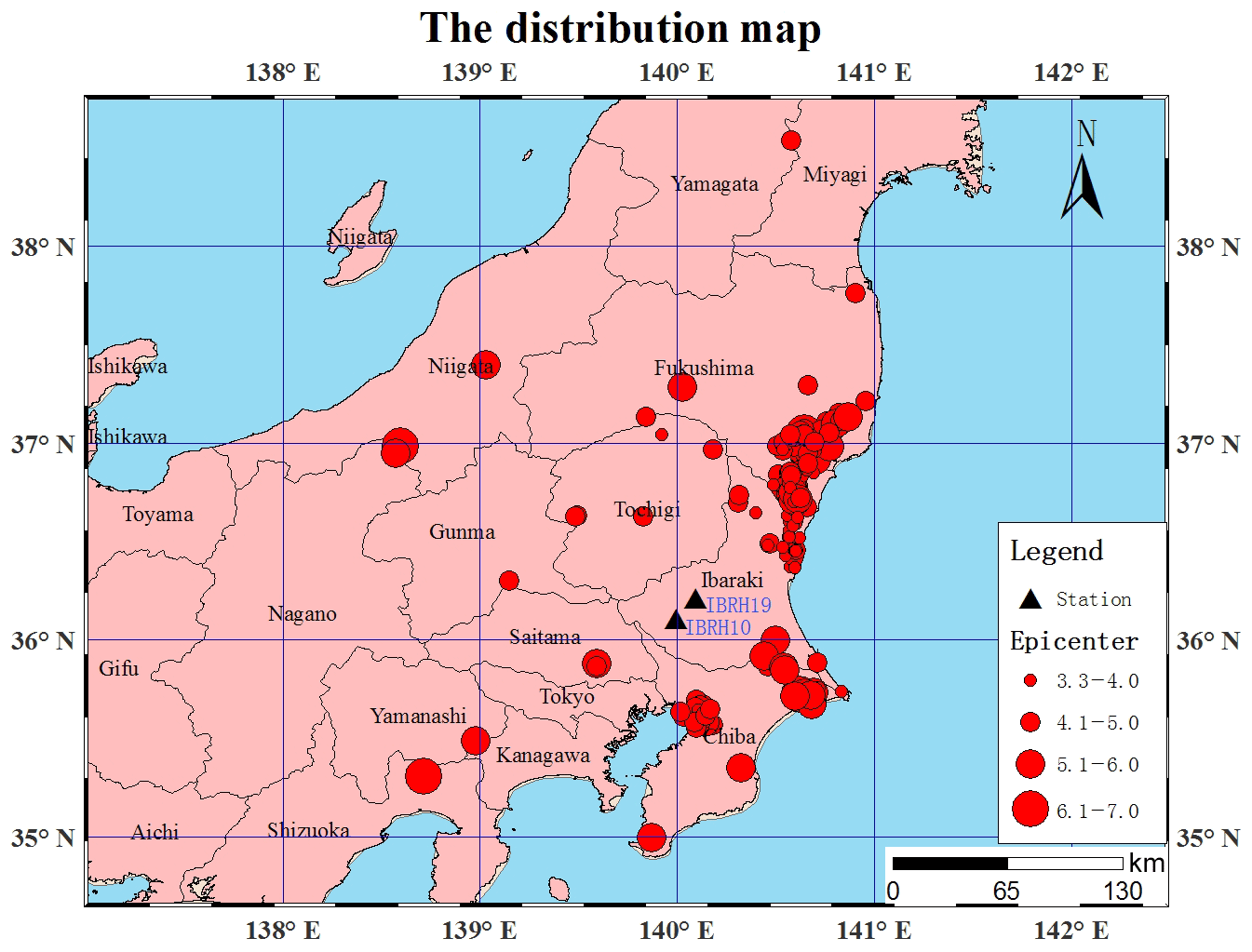
Figure 1The station and epicenter distribution map used for this research.
Source parameters, including the hypocenter location and magnitude, are determined within a few seconds after an earthquake occurs. Then the ground motion is estimated based on these parameters. While the EEW system uses a few parameters, parameter uncertainty leads to another error in the ground motion prediction. A new method was proposed by Hoshiba (2013). This method predicts ground motion using ground motion observed at front stations in the direction of incoming waves. The idea of this method was shown in Fig. 2. In this method, the observed information is sent directly forward to the target point. The core idea of this method is that the frequency-dependent site amplification factor can be reproduced by a casual recursive filter based on the historical relative spectral ratio between two stations. In this method the far-field simulated waveform can be obtained by real-time filtering of the observed waveform recorded in the front detection station.
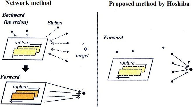
Figure 2Comparison of the method proposed by Hoshiba with the network method (modified after Hoshiba, 2013).
Seismic ground motion is often modeled by convolution of the source, propagation, and site amplification factors. Site amplification factors play an important role in determining seismic wave amplitude other than the propagation effect and source effect. Usually, the site amplification factor was evaluated in the frequency domain. However, for earthquake early warning systems, it is not suitable, as this procedure needs some length of windowed waveform for fast Fourier transform (FFT) in the frequency domain. In many previous studies, site amplification factors are estimated using the following equation (Iwata and Irikura, 1988):
where f is frequency in hertz; Okl(f), Sk(f), Gl(f), and Tkl(f) represent the observed seismic spectrum from event k at site l, the source spectrum characterizing the event k, the site amplification factor at site l, and the propagation factor between event k and site l, respectively; and f is the frequency of the seismic waves.
The frequency-dependent relative site amplification factors are assumed to be modeled by the following linear system of first-order and second-order filters:
where N and M stand for the numbers of the first-order and second-order filters, respectively, and s=iω. Here ω values are angular frequencies, and h values are damping factors that characterize the frequency dependence. represents a damping oscillation (Hoshiba, 2013). G0, ω1n, ω2n, ω1m, and ω2m are estimated for given values of N and M by using the least-squares method on logarithmic scales. We focus on the amplitude characteristics, ignoring phase characteristics. The bilinear transform (also known as Tustin's method) is introduced as
which is used in digital signal processing and the discrete-time control theory to transform continuous-time system representations into discrete time. Then the pre-warping equation,
is applied to ω1n, ω2n, ω1m, and ω2m. Next the transfer function F(z) is obtained, where ΔT is the sampling interval of the digital waveforms and z=exp(sΔT). Equation (3) and (4) are the necessary procedures for obtaining the coefficients of a causal recursive filter for real-time processing.
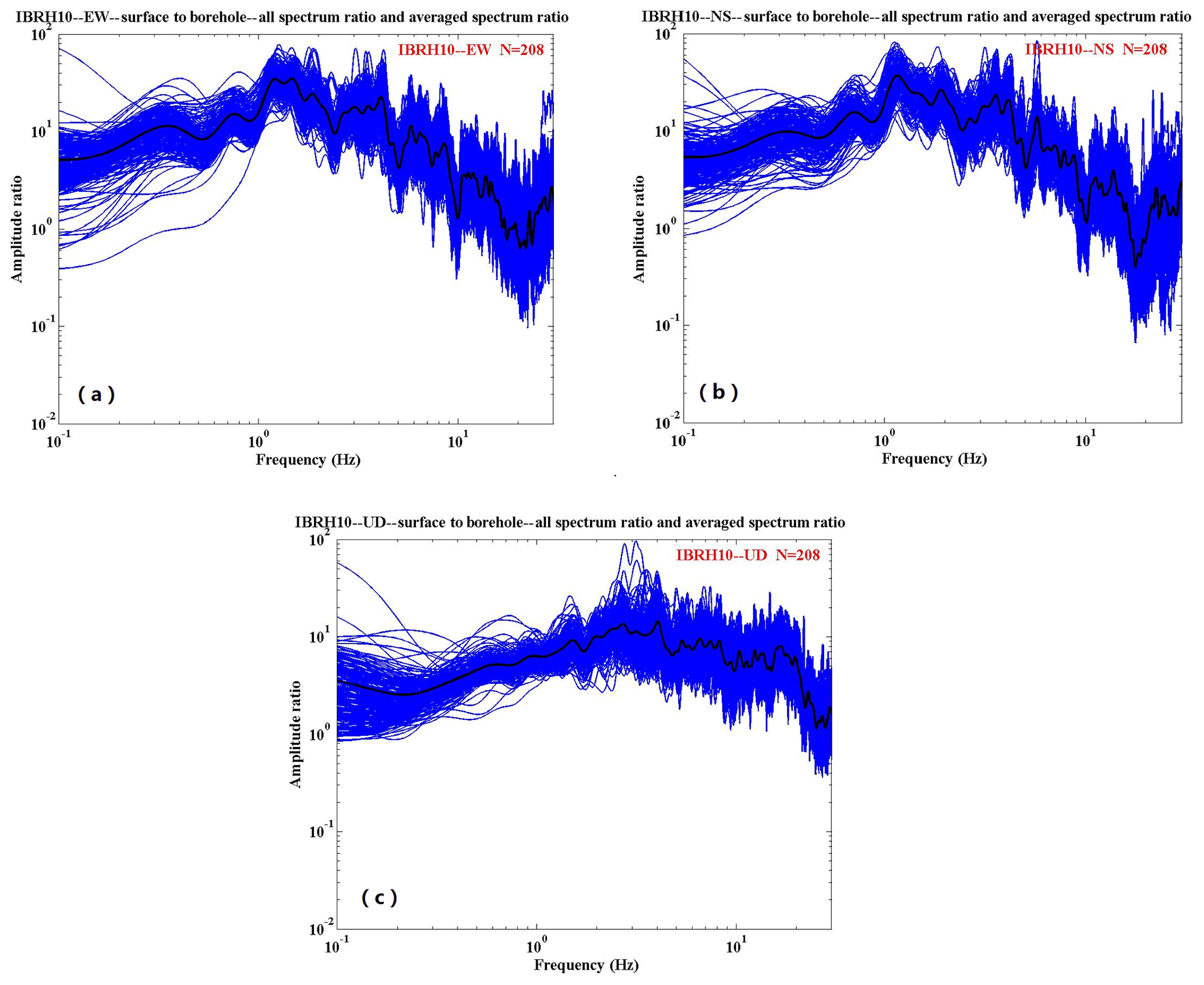
Figure 3Surface-to-borehole spectral ratios at IBRH10: (a) EW2 ∕ EW1, (b) NS2 ∕ NS1, and (c) UD2 ∕ UD1. The blue lines stand for the spectra ratio for every earthquake event, and the black line stands for the average spectra ratio for all the events.
4.1 Spectral ratios
We use the strong motion data recorded by IBRH10 and IBRH19 during these 208 earthquakes. The spectral ratio results obtained are shown in Fig. 3a to 5f. The Parzen window with a 0.3 Hz bandwidth was used to smooth the spectra. The spectral ratios of the east–west (EW) component and north–south (NS) component of IBRH10 have similar tendencies. The ratio is approximately 30 at around 1.3–1.5 Hz, whereas it is less than 2 at around 20 Hz (Fig. 3a and b). The spectral ratio of the up–down (UD) component of IBRH10 is approximately 10 at around 2–3 Hz, whereas it is less than 2 at around 25 Hz (Fig. 3c).The spectral ratios of the EW component and NS component of IBRH19 also have similar tendencies. It is approximately 6 at around 5 Hz and 4 at 13 Hz, whereas it is less than 2 at less than 2 Hz (Fig. 4a and b). The spectral ratio of the UD component of IBRH19 is approximately 5 at 5 Hz and 4 at 25 Hz, whereas it is less than 2 at around 3 Hz (Fig. 4c). The spectral ratio of the borehole component of IBRH10 to IBRH19 is almost flat, as this ratio is calculated from bedrock to bedrock. The maximum site amplification is 2.5 at about 20 Hz, and the spectral ratio is nearly 1 at the rest of the frequencies (Fig. 5a, c, and e). The spectral ratios of the EW component and NS component of the IBRH10 surface to the IBRH19 surface are approximately 20 at 1 to 2 Hz, whereas the ratio is less than 1 from 17 to 30 Hz (Fig. 5b and d). The spectral ratio of the UD component of the IBRH10 surface to the IBRH19 surface is approximately 10 at 1.5 Hz, whereas it is less than 1 from 22 to 30 Hz (Fig. 5f).
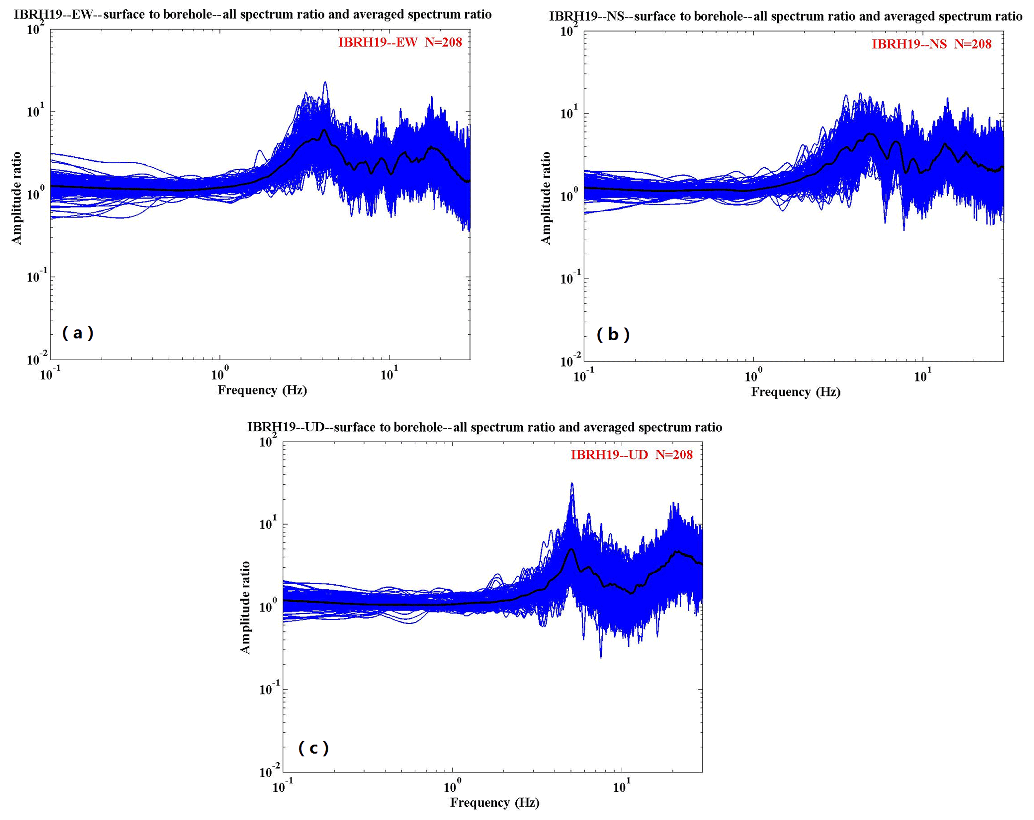
Figure 4Surface-to-borehole spectral ratios at IBRH19: (a) EW2 ∕ EW1, (b) NS2 ∕ NS1, and (c) UD2 ∕ UD1. The blue lines stand for the spectra ratio for every earthquake event, and the black line stands for the average spectra ratio for all the events.
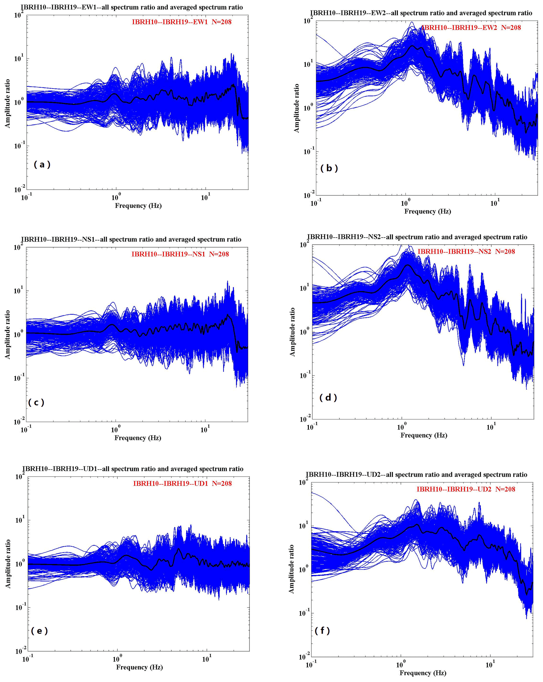
Figure 5Spectral ratios of IBRH10 to IBRH19 for (a) EW1, (b) EW2, (c) NS1, and (d) NS2. The blue lines stand for the spectra ratio for every earthquake event, and the black line stands the average spectra ratio for all the events. (e) UD1. (f) UD2. The blue lines stand for the spectra ratio for every earthquake event, and the black line stands for the average spectra ratio for all the events.
4.2 Simulation from borehole to surface
Firstly, we make the simulation from the borehole to the surface, although it is not useful for the earthquake early warning system. However, it could be used to make a full evaluation of this method. We use the strong motion data recorded by the IBR10 borehole sensor to simulate the surface station acceleration waveforms and spectrum. Figure 6a to d show the simulation results for the M4.5 earthquake which occurred on 21 November 2009. The information about the site amplification factors and the increment of seismic intensity are summarized in Table 1. In the table, amp., obs., sim., comp., res., surf., and boh. are the abbreviations of amplification, observation, simulation, component, residual, surface, and borehole respectively.
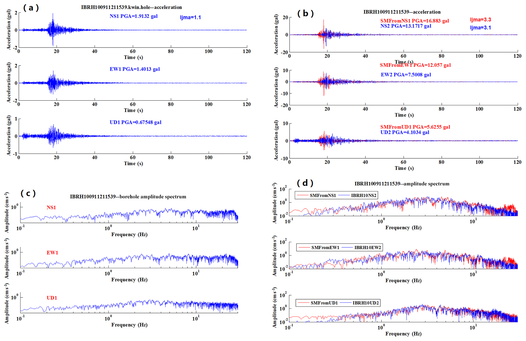
Figure 6An example of the results of simulation for IBRH100911211539: (a) the observed acceleration at the borehole, (b) the observed surface acceleration waveform (blue) compared with the simulated one (red), (c) the spectra of the observed borehole record, and (d) the spectra of the observed surface record (blue) compared with the simulated one (red).
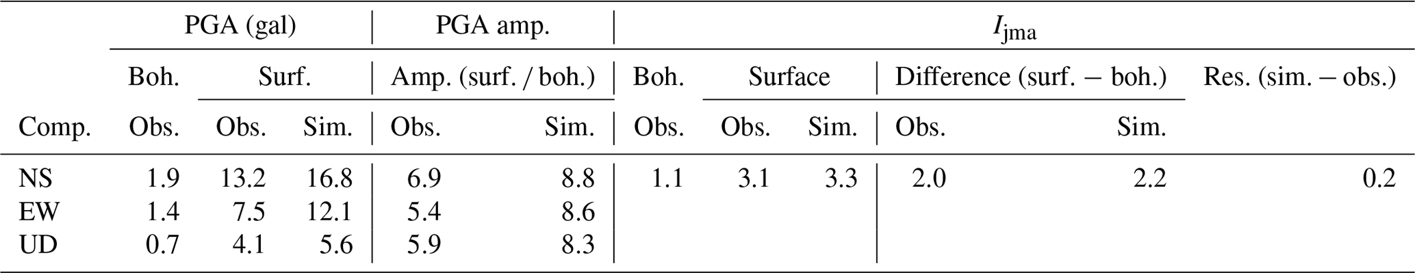
Figure 7a to d show the simulation results for the M4.6 earthquake which occurred on 7 December 2012. The information about the site amplification factors and the increment of seismic intensity are summarized in Table 2.
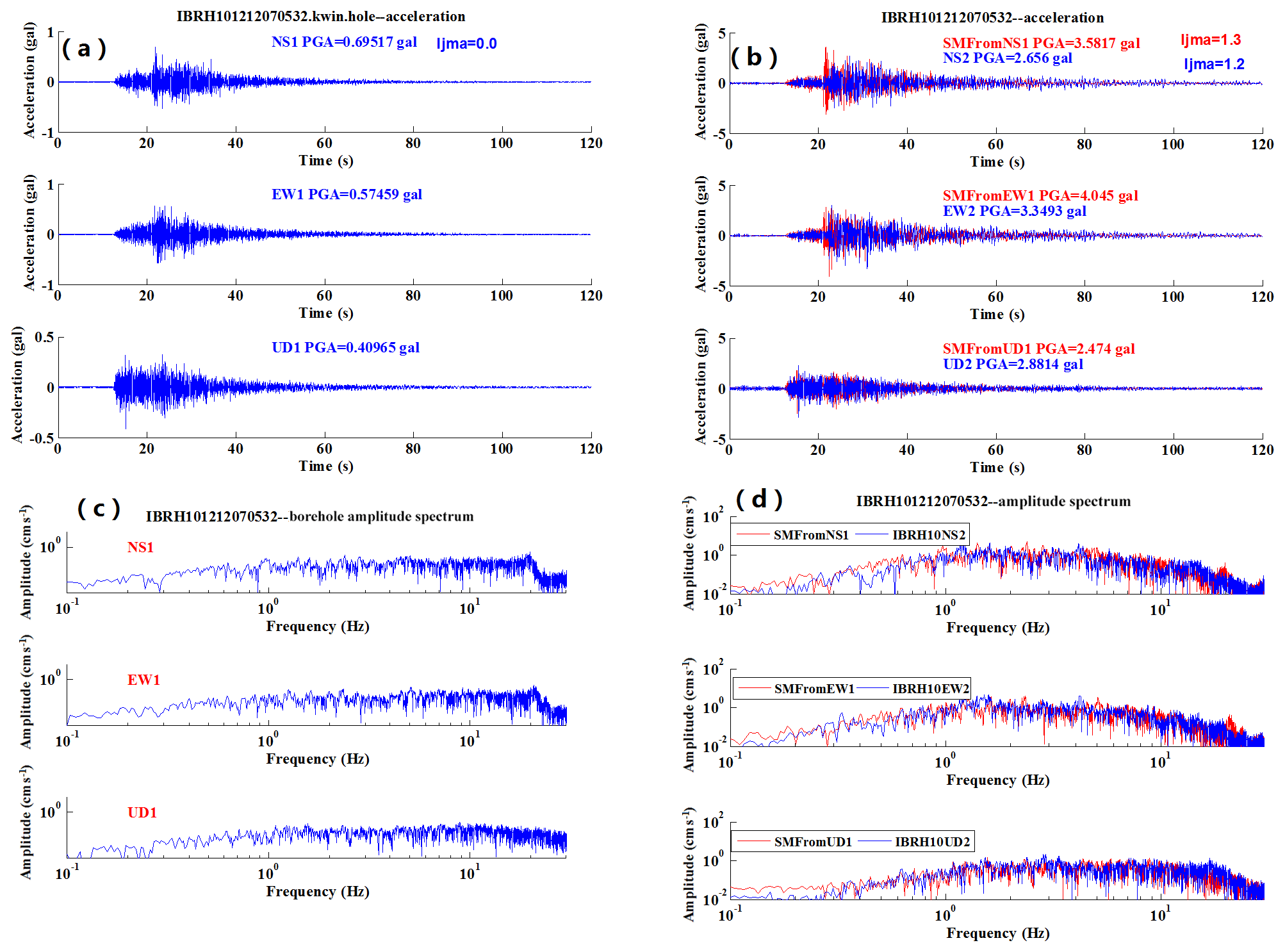
Figure 7An example of the results of simulation for IBRH101212070532: (a) the observed acceleration at the borehole, (b) the observed surface acceleration waveform (blue) compared with the simulated one (red), (c) the spectra of the observed borehole record, and (d) the spectra of the observed surface record (blue) compared with the simulated one (red).

For these two examples, comparing the simulated acceleration and spectrum with the observed acceleration and spectrum of the surface records, the results were simulated well. The different amplifications of maximum acceleration between Tables 1 and 2 reflect the differences of the frequency contents of the incident waveforms that cannot be reproduced by a scalar site amplification factor (e.g., amplification of peak ground acceleration or peak ground velocity or increment of seismic intensity).
The seismic intensity is calculated according to the method described in the paper (Yamazaki et al., 1998). Figure 8 shows the seismic-intensity residuals. The average seismic-intensity residual of these 208 earthquakes is 0.139. The standard deviation of the difference is 0.254; 98.6 % of the seismic-intensity residuals are less than 0.5, and 100 % of the seismic-intensity residuals are less than 1. As the minimum resolution for the seismic calculation is 0.1∘, it is reasonable that we consider that these simulations show good performance.
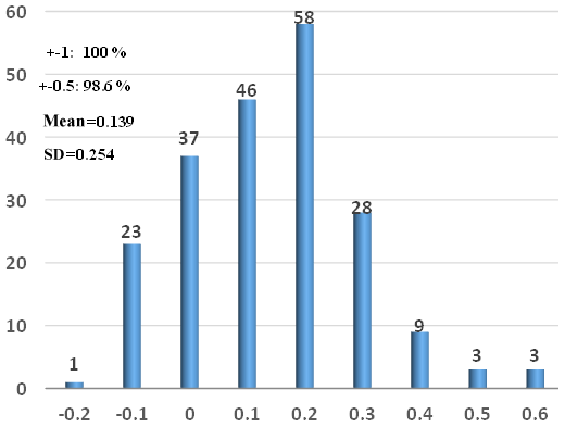
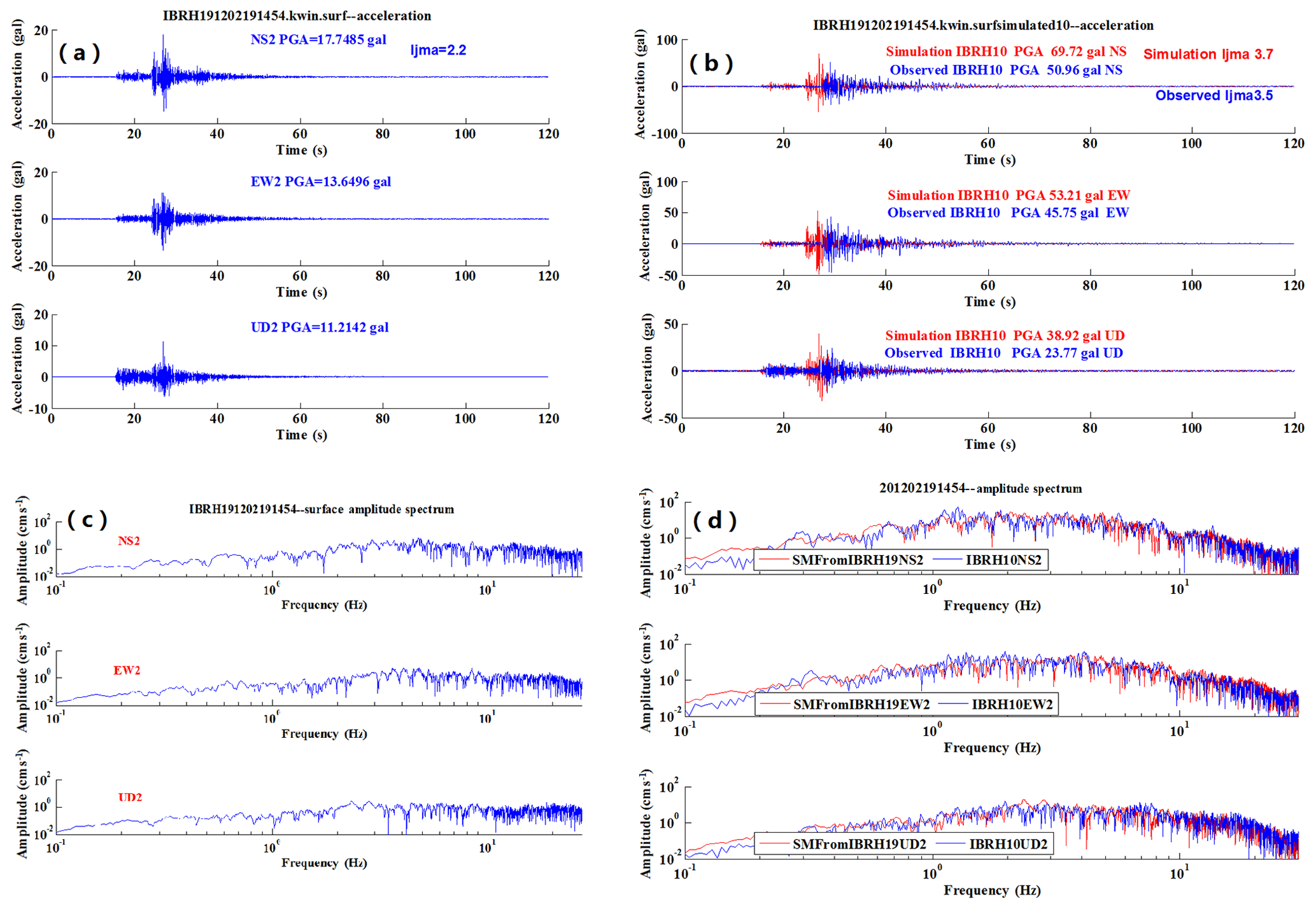
Figure 9An example of simulation from IBRH19 (surface) to IBRH10 (surface) for the earthquake 201202191454: (a) the observed surface acceleration for IBRH19, (b) the observed surface acceleration waveform (blue) compared with the simulated one (red), (c) the spectral ratio of observed surface record for IBRH19, and (d) the observed spectra of surface record at IBRH10 (blue) compared with the simulated one (red).
4.3 Simulation between front-detection station and far-field station
Then, using the surface strong motion data of IBRH19, we get simulated waveforms for IBRH10. Figure 9a–d show the simulation results for the M5.2 earthquake which occurred on 19 February 2012. The information about site amplification factors and the increment of seismic intensity is summarized in Table 3.
Table 3Information for M5.2 earthquake (IBRH10 and IBRH19 for 201202191454).
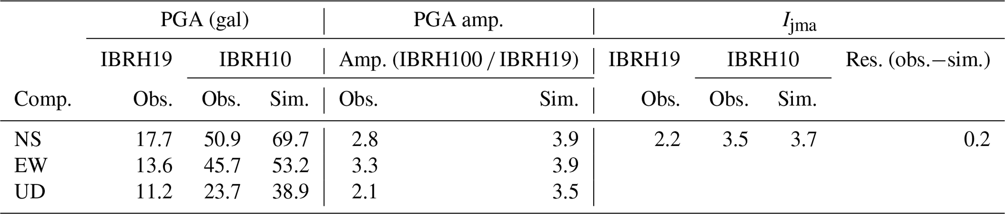
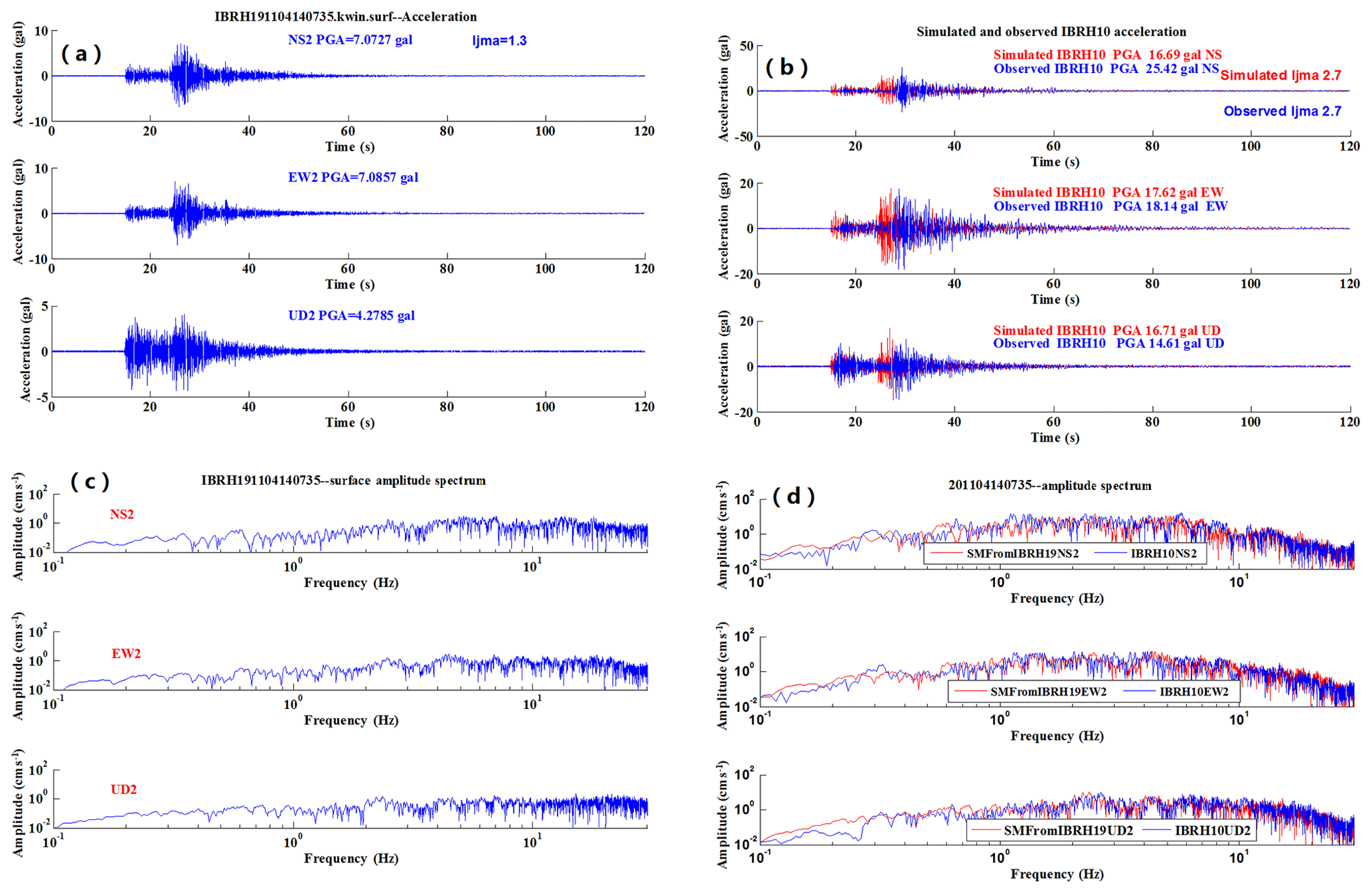
Figure 10An example of simulation from IBRH19 (surface) to IBRH10 (surface) for the earthquake 201104140735: (a) the observed surface acceleration for IBRH19, (b) the observed surface acceleration waveform (blue) compared with the simulated one (red), (c) the spectral of observed surface record for IBRH19, and (d) the observed spectra of surface record at IBRH10 (blue) compared with the simulated one (red).
The simulation results for the M5.1 earthquake that occurred on 14 April 2011 are shown in Fig. 10a–d. The comparison information about the site amplification factors and the increment of seismic intensity is summarized in Table 4.
Table 4Information for M5.1 earthquake (IBRH10 and IBRH19 for 201104140735).

Comparing the observed the surface record acceleration and spectrum with the simulated acceleration and spectrum shows that the simulation results are good. The acceleration amplification factors for the M5.2 earthquake which occurred on 19 February 2012 are 3.9, 3.9, and 3.5, while the acceleration amplification factors for the M5.1 earthquake which occurred on 14 April 2011 are 2.4, 2.5, and 3.9. Comparing the simulation results for these two earthquakes, the different amplification of acceleration between Tables 3 and 4 shows the different frequent content of the waveforms that cannot be reproduced by a scalar site amplification method.
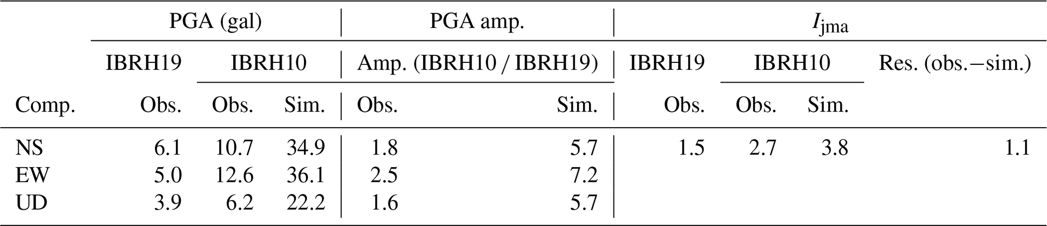
Although most of the simulation results show good performance, cases exist in which the simulation did not work well. For example, Fig. 11a–d show the simulation results for the M5.3 earthquake that occurred on 16 March 2011. The information about the site amplification factors and the increment of seismic intensity is summarized in Table 5. Comparing the observed acceleration and spectra with the simulated acceleration and spectra indicates that the simulation did not work well for the M5.3 earthquake that occurred on 16 March 2011.
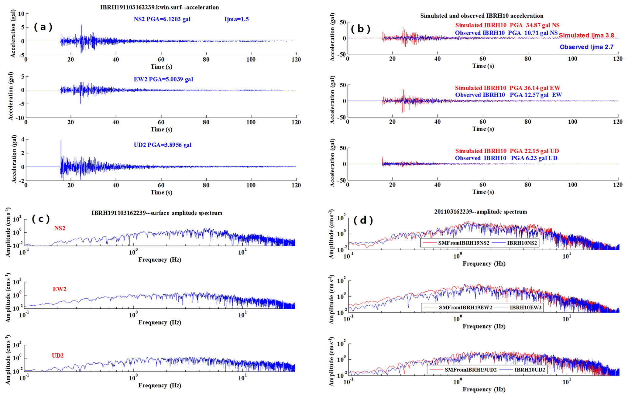
Figure 11An example of simulation from IBRH19 (surface) to IBRH10 (surface) for the earthquake 201103162239: (a) the observed surface acceleration for IBRH19, (b) the observed surface acceleration waveform (blue) compared with the simulated one (red), (c) the spectral ratio of observed surface record for IBRH19, and (d) the observed spectra of surface record at IBRH10 (blue) compared with the simulated one (red).
Table 5Information for M5.3 earthquake (IBRH10 and IBRH19 for 201103162239).
The seismic intensity is calculated according to the method described in the paper (Yamazaki et al., 1998). Figure 12 shows the seismic-intensity residual. The average seismic-intensity residual is 0.35 for our whole data set. The standard deviation of the seismic-intensity residual is 0.36; 69.7 % of the seismic-intensity residual is less than 0.5, and 98.1 % of the seismic-intensity residual is less than 1. Japan Meteorological Agency used the amplification factor relative to velocity (ARV) method (amplitude ratio of peak ground velocity at the ground surface relative to the engineering bedrock of averaged S-wave velocity – 700 m s−1) based on topographic data. Iwakiri et al. (2011) proposed the station correction method. The station correction method is based on site amplifications obtained empirically from observed seismic-intensity data.
We compared the performance of this method with the ARV method and station correction method. For the ARV method and station correction method, the seismic-intensity residual within ±0.5 is 55 % and 59 %, respectively. The seismic-intensity residual within ±1 is 84 % and 93 %, respectively, for the ARV method and station correction method. The comparison results between different methods are shown in Table 6. The statistical 1∘ seismic-intensity error of the current JMA EEW system (Japan Meteorological Agency, 2018) was shown in Fig. 13. The average 1∘ seismic-intensity error is 74.74 % for all 11 years of data. The best case is 93.7 % in 2017, and the worst case is 34.6 % in 2010. From the analysis mentioned above, we can conclude that this method could improve the accuracy of the seismic-intensity estimation. It highly improves the accuracy of predicting ground motion in real time and could be used in the earthquake early warning system.
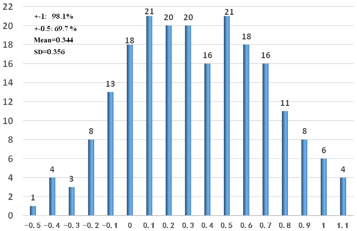
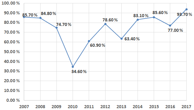
Figure 13The percent ratio diagram for 1∘ seismic-intensity error in the current Japan EEW system.

Through comparing different simulation cases, one can easily see that the frequency-dependent correction of the site amplification factor could produce different amplification factors for different earthquakes. It could produce the frequency-dependent site amplification factor and highly improves situations in which scalar-value site amplification methods could not produce different amplification factors for different earthquakes. It skips the procedure to calculate the EEW magnitude and epicenter distance or hypocenter distance using the starting portion of the waveform. We can obtain the waveform in real time at the target station. It highly improves the accuracy of predicting ground motion in real time compared with the scalar-value site amplification factor. The simulation from the borehole to the surface is not suitable for earthquake early warning systems, but it proves that this method shows good performance for simulating waveforms of the target station in real time. For the purpose of earthquake early warning, we need to save a lot of lead time for warning the public, requiring the distance between two stations to be much larger. It means that the method has a relation to network density. We could use the frequency-dependent site implication factor to predict the seismic intensity more accurately in the seismic-intensity quick report system and earthquake early warning system with high network density. For the purposes of earthquake early warning, we need to use a large amount of historical ground motion records to model the relative site amplification and find the optional casual-filter parameter firstly. In the area with a sparse network and low seismicity, we could not get the relative site amplification easily because of a small number of strong motion records. We need to consider other methods for estimating the relative site amplification factor. We can adopt a method such as the coda normalization method (Phillips and Aki, 1986) or generalized spectrum inversion method (Iwata and Irikura, 1986; Kato et al., 1992).
There are cases in which some simulations did not work very well; 1.9 % of the seismic-intensity residuals are larger than 1. One of possible reasons is the azimuth dependency of site amplification (Cultrera et al., 2003). We did not consider azimuth dependency in designing the frequency-dependent filter for the site amplification factor. If we design multiple frequency-dependent correction filters for the site amplification factor regarding the azimuth dependency of site amplification, we would be able to predict the target ground motion more precisely. Another possible reason is the accuracy of the input relative spectral ratio. This situation may be improved by more precisely characterizing the input spectral ratio and complicated filter design. For example, we can use a large number of first- and second-order filters to model the spectral ratio, but it is more complicated and time-consuming for the hardware design when the number of filters grows larger. We need to make a trade-off between the accuracy of the input spectral ratio and the difficulty of the filter design.
This method pays attention to the amplitude characteristics and ignores the phase characteristics; there are a few papers on how to consider the phase in the earthquake early warning system. This situation may be improved with the seismic-interferometry method (Yamada et al., 2010). Because the site amplification factor was assumed to be a linear system, the nonlinearity of weak ground motion and strong ground motion (Noguchi et al., 2012) was not taken into consideration in this study. More research is needed to solve these problems.
In this paper, we evaluate the infinite impulse recursive filter method that models the relative site amplification factor by historical strong ground motion data and then implements the relative site amplification factor with the casual filter. First, we calculated the spectrum ratio for IBRH10 and IBRH19; then we obtained the surface simulated acceleration time series and spectrum for IBRH10 from borehole records at IBRH10. Similarly, we obtained the IBRH10-simulated surface acceleration time series and spectrum from the surface strong ground motion records of IBRH19. Lastly, we calculated the seismic-intensity residual between the observed data and simulated data and then compared the accuracy with the previous method and statistical report. This method highly improves the accuracy of predicting ground motion in real time. The results show the following.
-
The spectra ratio is calculated between the borehole record and surface record from the same station. Then we use the infinite impulse recursive filter method to model our relative spectra ratio. The average seismic-intensity residual of these earthquakes is 0.139. The standard deviation of these seismic-intensity residuals is 0.254; 98.6 % of these seismic-intensity residuals are less than 0.5, and 100 % of these seismic-intensity residuals are less than 1.
-
The spectra ratio is calculated between IBRH10 and IBRH19 surface records. Similarly, we use the infinite impulse recursive filter method to model the relative spectra ratio between two stations. The average seismic-intensity residual of these earthquakes is 0.35. The standard deviation of these seismic-intensity residuals is 0.36; 69.7 % of these seismic-intensity residuals are less than 0.5, and 98.1 % of these seismic-intensity residuals are less than 1. This method shows better performance than the ARV method and station correction method. The average 1∘ seismic-intensity error of all 11 years of statistical data of the current Japan Meteorological Agency earthquake early warning system is 74.74 %. This method also shows better performance than the current operational Japan Meteorological Agency earthquake early warning system. This method highly improves the accuracy of predicting ground motion in real time.
The hypocenter parameters, including the origin time, location of hypocenter, and magnitude, used in this study, which were routinely determined by JMA, were obtained from the JMA seismic catalog. The KiK-net strong motion data can be downloaded from the NIED website (http://www.kyoshin.bosai.go.jp/, last access: 23 September 2019). We thank JMA and NIED for their hard work.
QX completed the core work and wrote the text content, QM and JZ were the technical directors in chief, and HY supervised the strong motion data processing and related analysis. All authors discussed the editor opinions and revised the paper.
The authors declare that they have no conflict of interest.
We thank Toshiaki Yokoi (BRI) and Mitsuyuki Hoshiba (MRI) for supervising Quancai Xie and providing useful suggestions for this study. We also thank Toshihide Kashima(BRI) for providing the program that we used for calculating the JMA seismic intensity.
This work is partially supported by the Scientific Research Fund of the Institute of Engineering Mechanics, China Earthquake Administration (grant no. 2019B06), National Key Research and Development Program of China (grant no. 2018YFE0109800), National Natural Science Foundation of China (grant no. 41874059), and Seismological Science and Technology Spark Project (grant no. XH19071).
This paper was edited by Filippos Vallianatos and reviewed by Hao Chen and three anonymous referees.
Alcik, H., Ozel, O., Apaydin, N., and Erdik, M.: A study on warning algorithms for Istanbul earthquake early warning system, Geophys. Res. Lett., 36, L00B05, https://doi.org/10.1029/2008GL036659, 2009.
Allen, R. M. and Kanamori, H.: The potential for earthquake early warning in southern California, Science, 300, 786–789, 2003.
Allen, R. M., Brown, H., Hellweg, M., Khainovski, O., Lombard, P., and Neuhauser, D.: Real-time earthquake detection and hazard assessment by ElarmS across California, Geophys. Res. Lett., 36, L00B08, https://doi.org/10.1029/2008GL036766, 2009.
Bose, M., Hauksson, E., Solanki, K., Kanamori, H., and Heaton, T. H.: Real-time testing of the on-site warning algorithm in southern California and its performance during the July 29, 2008 Mw 5.4 Chino Hills earthquake, Geophys. Res. Lett., 36, L00B03, https://doi.org/10.1029/2008GL036366, 2009.
Cultrera, G., Rovelli, A., Mele, G., Azzara, R., Caserta, A., and Marra, F.: Azimuth-dependent amplification of weak and strong ground motions within a faultzone (Nocera Umbra, central Italy), J. Geophys. Res., 108, 2156, https://doi.org/10.1029/2002JB001929, 2003.
Erdik, M., Fahjan, Y., Ozel, O., Alcik, H., Mert, A., and Gul, M.: Istanbul earthquake rapid response and the early warning system, B. Earthq. E., 1, 157–163, 2003.
Espinosa-Aranda, J. M., Jimenez, A., Ibarrola, G., Alcantar, F., Aguilar, A., Inostroza, M., and Maldonado, S.: Mexico City Seismic Alert System, Seismol. Res. Lett., 66, 42–52, 1995.
Espinosa-Aranda, J. M., Cuellar, A., Garcia, A., Ibarrola, G., Islas, R., Maldonado, S., and Rodriguez, F. H.: Evolution of the MexicanSeismic Alert System (SASMEX), Seismol. Res. Lett., 80, 694–706, 2009.
Horiuchi, S., Negishi, H., Abe, K., Kamimura, A., and Fujinawa, Y.: An automatic processing system for broadcasting earthquake alarms, B. Seismol. Soc. Am., 95, 708–718, 2005.
Horiuchi, S., Horiuchi, Y., Yamamoto, S., Nakajima, H., Wu, C., Rydelek, P. A., and Kachi, M.: Home seismometer for earthquake early warning, Geophys. Res. Lett., 36, L00B04, https://doi.org/10.1029/2008GL036572, 2009.
Hoshiba, M., Kamigaichi, O., Saito, M., Tsukada, S., and Hamada, N.: Earthquake early warning starts nationwide in Japan, EOS T. Am. Geophys. Un., 89, 73–80, 2008.
Hoshiba, M., Iwakiri, K., Hayashimoto, N., Shimoyama, T., Hirano, K., Yamada, Y., Ishigaki, Y., and Kikuta, H.: Outline of the 2011 off the Pacific coast of Tohoku Earthquake (Mw 9.0), Earth Planets Space, 63, 547–551, 2011.
Hoshiba, M.: Real Time Correction of Frequency-Dependetnt Site Amplification Factors for Application to Earthquake Early Warning, B. Seismol. Soc. Am., 103, 3179–3188, 2013.
Hsiao, N. C., Wu, Y. M., Shin, T. C., Zhao, L., and Teng, T. L.: Development of earthquake early warning system in Taiwan, Geophys. Res. Lett., 36, L00B02, https://doi.org/10.1029/2008GL036596, 2009.
Ionescu, C., Bose, M., Wenzel, F., Marmureanu, A., Grigore, A., and Marmureanu, G.: Early warning system for deep Vrancea (Romania) earthquakes, in: Earthquake Early Warning Systems, edited by: Gasparini, P., 2007.
Iwata, T. and Irikura, K.: Separation of source, propagation and site effects from observed S-waves, Zisin II, 39, 579–593, 1986 (in Japanese with English abstract).
Iwata, T. and Irikura, K.: Source parameters of the 1983 earthquake sequence, J. Phys. Earth, 36, 155–184, 1988.
Iwakiri, K., Hoshiba, M., Nakamura, K., and Morikawa, N.: Improvement in the accuracy of expected seismic intensities for earthquake early warning in Japan using empirically estimated site amplification factors, Earth Planets Space, 63, 57–69, 2011.
Japan Meteorological Agency: The EEW statistical report on the Japan Meteorological Agency EEW system [EB/0L], http://www.data.jma.go.jp/svd/eqev/data/study-panel/eew-hyoka/10/shiryou1-1.pdf (last access: 20 November 2018), 2018 (in Japanese).
Kamigaichi, O.: JMA earthquake early warning, Journal of the Japan Association for Earthquake Engineering, 4, 134–137, 2004.
Kato, K., Takemura, M., Ikeura, T., Urao, K., and Uetake, T.: Preliminary analysis for evaluation of local site effects from strong motion spectra by an inversion method, J. Phys. Earth, 40, 175–191, 1992.
Nakamura, H., Horiuchi, S., Wu, C., Yamamoto, S., and Rydelek, P. A.: Evaluation of the real-time earthquake information system in Japan, Geophys. Res. Lett., 36, L00B01, https://doi.org/10.1029/2008GL036470, 2009.
Noguchi, S., Sato, H., and Sasatani, T: Characterization of nonlinear site response based on strong motion records at K-NET and KiK-net stations in the east of Japan., Proc. of 15th World Conference on Earthquake Engineering, Lisbon, Portugal, 24–28 September 2012, abstract number 3846, 2012.
Okada, T., Ashiya, K., Tsukuda, A., Sato, S., Ohtake, T., and Nozaka, D.: A new method of quickly estimating epicentral distance and magnitude from a single seismic record, B. Seismol. Soc. Am., 93, 526–532, 2003.
Peng, H. S., Wu, Z. L., Wu, Y. M., Yu, S. M., Zhang, D. N., and Huang, W. H.: Developing a Prototype Earthquake Early Warning System in the Beijing Capital Region, Seismol. Res. Lett., 82, 394–403, https://doi.org/10.1785/gssrl.82.3.394, 2011.
Phillips, W. S. and Aki, K.: Site amplification of coda waves from local earthquakes in central California, B. Seismol. Soc. Am., 76, 627–648, 1986.
Wenzel, F., Onescu, M., Baur, M., and Fiedrich, F.: An early warning system for Bucharest, Seismol. Res. Lett., 70, 161–169, 1999.
Wu, Y. M. and Teng, T. L.: A virtual subnetwork approach to earthquake early warning, B. Seismol. Soc. Am., 92, 2008–2018, 2002.
Yamada, M., Mori, J., and Ohmi, S.: Temporal changes of subsurface velocities during strong shaking as seen from seismic interferometry, J. Geophys. Res., 115, B03302, https://doi.org/10.1029/2009JB006567, 2010.
Yamazaki, F., Noda, S., and Meguro, K..: Developments of early earthquake damage assessment systems in Japan, Proc. of 7th International Conference on Structural Safety and Reliability, 1573–1580, 1998.
Zollo, A., Lancieri, M., and Nielsen, S.: Earthquake magnitude estimation from peak amplitudes of very early seismic signals on strong motion records, Geophys. Res. Lett., 33, L23312, https://doi.org/10.1029/2006GL027795, 2006.
Zollo, A., Iannaccone, G., Lancieri, M., Cantore, L., Convertito, V., Emolo, A., Festa, G., Gallovic, F., Vassallo, M., Martino, C., Satriano, C., and Gasparini, P.: Earthquake early warning system in southern Italy: Methodologies and performance evaluation, Geophys. Res. Lett., 36, L00B07, https://doi.org/10.1029/2008GL036689, 2009.