the Creative Commons Attribution 4.0 License.
the Creative Commons Attribution 4.0 License.
 | 17 Oct 2019
Identifying a transition climate zone in an arid river basin using the evaporative stress index
Yongqiang Liu
Lu Hao
Decheng Zhou
Cen Pan
Peilong Liu
Zhe Xiong
Ge Sun
Aridity indices have been widely used in climate classification. However, there is not enough evidence for their ability in identifying the multiple climate types in areas with complex topography and landscape, especially in those areas with a transition climate. This study compares a traditional meteorological aridity index (AI), defined as the ratio of precipitation (P) to potential evapotranspiration (PET), with a hydrological aridity index, the evaporative stress index (ESI) defined as the ratio of actual evapotranspiration (AET) to PET in the Heihe River Basin (HRB) of arid northwestern China. PET was estimated using the Penman–Monteith and Hamon methods. The aridity indices were calculated using the high-resolution climate data simulated with a regional climate model for the period of 1980–2010. The climate classified by AI shows a climate type for the upper basin and a second type for the middle and lower basin, while three different climate types are found using ESI, each for one river basin, indicating that only ESI is able to identify a transition climate zone in the middle basin. The difference between the two indices is also seen in the interannual variability and extreme dry/wet events. The magnitude of variability in the middle basin is close to that in the lower basin for AI, but different for ESI. AI had a larger magnitude of the relative interannual variability and a greater decreasing rate from 1980 to 2010 than ESI, suggesting the role of local hydrological processes in moderating extreme climate events. Thus, the hydrological aridity index is better than the meteorological aridity index for climate classification in the arid Heihe River Basin.
- Article
(7755 KB) - Full-text XML
- BibTeX
- EndNote


Aridity indices combine one or several variables (indicators) into a single numerical value to measure water deficit over long periods (e.g., 30 years or longer) (Wilhite and Glantz, 1985; Zargar et al., 2011). Aridity indices are a useful tool for climate classification (https://en.wikipedia.org/wiki/Climate_classificationin, last access: 8 October 2019). In comparison with comprehensive tools such as the Köppen climate classification (Peel et al., 2007), aridity indices do not need complex information on the properties of ecosystems and therefore are used more easily and often at local and regional scales.
Aridity indices can be categorized into different types including meteorological and hydrological indices, which could be simply considered to be a lack of water due to anomalous atmospheric and land-surface conditions, respectively. Precipitation, temperature, and humidity are atmospheric conditions often used to estimate meteorological aridity indices. The earliest aridity index, developed more than a century ago, reflects the effects of the thermal regime and the amount and distribution of precipitation in determining the native vegetation possible in an area. By the middle of the 20th century, attention turned to precipitation and potential evaporation (Huschke, 1959). A typical index of this type, the Budyko-type aridity index (AI) (Budyko, 1974), for example, uses annual averages of precipitation and potential evapotranspiration (PET), which is mainly determined by temperature.
Land-surface conditions such as streamflow, runoff, and actual evapotranspiration are often used to estimate hydrological aridity indices (Maliva and Missimer, 2012). The evaporative stress index (ESI), for example, defines dryness degree based on the ratio of actual evapotranspiration (AET) to PET over both short and long periods. A relatively low ESI indicates water limitation to plants, and the actual rate is way below the PET. In contrast, a relatively high ESI indicates freely available water with the AET rate approaching or close to the PET. The ESI has been used to evaluate the irrigation need for crop growth and land classification (Yao, 1974). The ESI was used recently to evaluate water stress using remotely sensed hydrological and ecological properties (Anderson et al., 2016).
There are many similarities between aridity indices and drought indices, which measure water deficit over short periods (such as months, seasons, and years). Drought indices also are categorized into meteorological, hydrological, and other types. The percent of normal (PN) and standardized precipitation index (SPI) (McKee et al., 1993) are simply based on precipitation and can be used to measure anomalies of a period over various lengths. The Palmer drought severity index (PDSI) (Palmer, 1965) and Keetch–Byram drought index (KBDI) model (Keetch and Byram, 1968) are based on water supply and demand estimated mainly using precipitation and temperature (Guttman, 1999). Both PDSI and KBDI depend on precedent daily or monthly values, making them specifically useful for a persistent event like drought. Among various hydrological drought indices, the streamflow drought index (SDI) (Nalbantis and Tsakiris, 2009) and surface water supply index (SWSI) (Shafer and Dezma, 1982) use streamflow as well as reservoir storage and precipitation to monitor abnormal surface water (Narasimhan and Srinivasan, 2005). The standardized runoff index (SRI) (Shukla and Wood, 2008) is standard normal deviate associated with runoff accumulated over a specific duration.
Large river basins at continental and subcontinental scales usually encompass multiple climate types related to complex topography and landscape. Climate is more humid in the upper basin near the river origins with high elevations and forest and/or permanent snow cover than the lower basin with low elevations and less vegetated lands. The climate could be extremely dry in parts of a watershed under a prevailing atmospheric high-pressure system. The subcontinental Colorado River watershed, for example, is dominated by cold and humid continental climate in the upper basin of the Rocky Mountains and cold semiarid or warm desert climate in the lower basin of the southern intermountains (the states of Utah and Nevada). This feature of multiple climate types is also seen in some smaller basins. The Heihe River Basin (HRB) in northwestern China, for example, has an area of 130 000 km2 with annual precipitation varying dramatically from about 500 mm in the upper basin of the Qilian Mountains with forest–meadow–ice covers in the south to less than 100 mm in the lower basin of the Alxa high plain with Gobi and sandy lands in the north. Climate types change from cold and humid continental to arid desert accordingly. The relative high precipitation in the humid upper basin supports forests and meadows and provides source water lower reach of the Heihe River. In contrast, water is a major limitation factor in the arid lower basin. In addition, more extreme weather conditions, especially droughts, occur in the arid lower basin. In the Colorado River basins, the reconstructed data show decadal periods of persistently low flows during the past centuries (Woodhouse et al., 2010). The drought severity in the new millennia has been the most extreme over a century (Cayan et al., 2010). The reconstructed precipitation series in the HRB indicates that droughts were much more frequent and lasted longer than floods in the past two centuries (Ren et al., 2010). Droughts occurred more often in the dry lower basin than the humid upper basin (Li, 2012). The watersheds with varied topography and landscape may have a transition climate zone between the two zones. In the HRB, for example, the Köppen climate classification, one of the most widely used climate classification techniques at large geographic scales and constructed based on the properties of ecosystems, latitude, and average and seasonal precipitation and temperature, shows polar tundra or boreal climate in the upper basin of the mountain regions in the south, arid desert climate in the lower basin in the north, and a transition zone of steppe climate in the middle. Identifying this transition zone and understanding its unique climate features are of both scientific and management significance. The complex topography in the upper basin and harsh climate in the lower basin make both regions unsuitable for human living. The transition zone however is relatively flat in comparison with the mountain region and less arid in comparison with the dryland region. It therefore provides a favorable condition for industrial and agricultural development. Also, the environmental conditions in this region are more dynamical and localized because of human-induced rapid and fragmental landscape changes.
ESI is similar to AI but more related to surface hydrology. However, unlike AI, ESI applications for climate classification have yet to be conducted. In addition, many studies have compared ESI with other drought indices in different climatic environments. For example, Otkin et al. (2013) compared the ESI with drought classification used by the U.S. Drought Monitor (USDM) (Svoboda et al., 2002) and found that the ESI anomalies led the USDM drought depiction by several weeks, and large ESI anomalies therefore were indicative of rapidly drying conditions. This finding was coincident with the droughts that occurred across the United States in recent years. Choi et al. (2013) compared the ESI with the Palmer drought severity index in a watershed of the Savannah River branch in the southeastern United States during 2000–2008. They found that the ability of the ESI to capture shorter term droughts was equal or superior to the PDSI when characterizing droughts for the watershed with a relatively flat topography dominated by a single land cover type. However, the differences between ESI and meteorological indices in capturing the spatial patterns under complex topography and environments are not well characterized and understood.
This study is to compare the capacity of the hydrological aridity index, ESI, and the meteorological aridity index, AI, in climate classification, especially in identifying a possible transition climate zone in the HRB. These two indices reflect the water (precipitation and evapotranspiration) and heat (radiation) properties on the ground surface without the need to obtain the complex vegetation and soil hydrological properties. The surface properties needed to calculate ESI and AI could be obtained from regional climate modeling, which was an approach used in this study. The analysis of the climate zones was made by comparing the spatial patterns and regional averages. Their temporal variations were also analyzed to understand the differences in the seasonal and interannual variability and long-term between ESI and AI.
2.1 Study region
The study region was the HRB and the adjacent areas (Fig. 1). The Heihe River originates from the Qilian Mountains in the northern edge of the Tibet Plateau and flows northward to the China–Russia border. The HRB spans between 98 and 101∘30′ E and 38 an 42∘ N. The upper HRB is within the mountains at an elevation of 2300–3200 m, mainly covered with forests and mountain meadows. The middle HRB is along the Hexi Corridor at an elevation of 1600–2300 m, mainly covered with piedmont steppe grass, crops, and residence and commercial uses. The lower HRB is in the Alxa high plain at an elevation of below 1600 m, mainly covered with Gobi and desert sands.

Figure 1The study region of the Heihe River Basin (red box) in China and the Köppen climate classification (from Peel et al., 2007).
Annual precipitation is over 400 mm in the upper basin, with the maximum of 800 mm at extremely high elevations, about 100–250 mm in the middle basin, and below 50 mm in many lower basin areas. The annual precipitation in the upper basin has high seasonal variability, and nearly 70 % of the total annual rainfall occurs from May to September (Gao et al., 2016). The upper basin generates nearly 70 % of the total river runoff, which supplies agricultural irrigation and benefits the social economy development in the middle and lower basin reaches (Yang et al., 2015; Chen et al., 2005). Annual mean temperature is about −4 ∘C in the upper basin, 7 ∘C in the middle basin, and nearly 9 ∘C in the lower basin.
2.2 Aridity indices
The meteorological aridity index is defined as AI = P/PET, where P and PET are daily precipitation and potential evapotranspiration, respectively. AI is a variant of the index originally defined by Budyko (1974), which is the ratio of annual PET to P. The average AI values were used to classify the arid, semiarid, semihumid (subhumid), and humid climate with the ranges of AI ≤ 0.2, 0.2 < AI ≤ 0.5, 0.5 < AI ≤ 1.3, and AI > 1.3, respectively (Ponce et al., 2000). The hydrological aridity index is defined as ESI = AET/PET, where AET is daily actual evapotranspiration. The ranges of average ESI values of ESI ≤ 0.1, 0.1 < ESI ≤ 0.3, 0.3 < ESI ≤ 0.6, and ESI > 0.6 were used to classify the arid, semiarid, semihumid, and humid climate, respectively (Yang, 2007). This approach agrees with Anderson (2011), which showed that the ESI values varying gradually from 0 to 1 correspond to several USDM drought levels from “exceptional drought” to “no drought” for each month from April to September across the continental US.
Two methods were used to estimate PET (mm d−1). One was the energy-balance-based FAO-56 Penman–Monteith equation (Allen et al., 1998):
where NRAD and G are net radiation and soil flux on the ground (MJm−2 d−1), T is air temperature (∘C), es and e are saturation and actual water vapor pressure (kPa), u2 is wind speed at 2 m above the ground (ms−1), Δ is the rate of change of es with respect to T (kPa/∘C), and γ is the psychrometric constant (kPa/∘C). The other method is the temperature based on the Hamon formula (Hamon, 1963):
where k is proportionality coefficient = 1 and N is daytime length. es is in 100 Pa here.
Monthly PET, precipitation, and actual evapotranspiration, obtained based on daily values, were used to calculate the aridity indices. It was assumed that daily PET = 0 if daily T < 0 ∘C. Their monthly PET was not used if PET = 0 for more than 10 d in a month. In this case, no aridity indices were calculated for the month. It was also assumed that daily ground energy was in balance, so , where H and L are sensible heat flux and potential heat constant.
A T test was conducted to obtain the statistical significance of the differences in the aridity index values between two Heihe River reaches. The data used in calculation and evaluation of the aridity indices are listed in Table 1.
Table 1The data used in calculation and evaluation of the aridity indices. H, AET, P, T, and e (RH) are sensible heat flux, actual evapotranspiration, precipitation, temperature, wind speed, and water vapor pressure (relative humidity). HRB stands for Heihe River Basin.

2.3 Regional climate modeling
The climatic and hydrological data used to calculate the aridity indices were created from a regional climate modeling using the Regional Integrated Environmental Modeling System (RIEMS 2.0) (Xiong and Yan, 2013). The simulation was conducted over the period of 1980–2010. The horizontal spatial resolution was 3 km. A unique feature with this simulation was that the model's parameters, including soil hydrological properties, were recalibrated based on observations and remote sensing data over the HRB that greatly improved the model's performance. The model evaluation indicated that the model was able to reproduce the spatial pattern and seasonal cycle of precipitation and surface T. The correlation coefficients between the simulated and observed pentad P were 0.81, 0.51, and 0.7 in the upper, middle, and lower HRB regions, respectively (p < 0.01).
The historical T and P observations during the simulation period at Yeniugou of the upper basin (38.25∘ N, 99.35∘ E, 3300 m a.s.l.), Zhangye of the middle basin (38.11∘ N, 100.15∘ E, 1484 m), and Dingxing of the lower basin (40.3∘ N, 99.52∘ E, 1177 m) were used to compare with the simulations. We also calculated SPI based on observed precipitation using a built-in function of the NCAR NCL (https://www.ncl.ucar.edu/, last access: 8 October 2019). The results with measured precipitation were used to evaluate the model performance in simulating drought conditions.
3.1 Simulated climate and hydrology
The spatial pattern of the simulated annual T averaged over the simulation period is featured by the large changes between basin reaches, increasing from about −15 ∘C in the tall mountains of the upper basin to over 10 ∘C in the deserts of the lower basin (Fig. 2). The simulated average annual P shows an opposite gradient, decreasing from about 2.5 mm d−1 in the mountains to less than 0.25 mm d−1 in the deserts (Fig. 2). The simulated NRAD decreases from west to east in the mountains, corresponding to an increasing trend in precipitation. NRAD is small in the northeastern section of the domain, probably due to large outgoing long-wave radiation related to clear and relative hot weather. The simulated average annual AET has a similar pattern to precipitation (Fig. 2). The spatial variability is much larger within the upper basin than the lower basin.
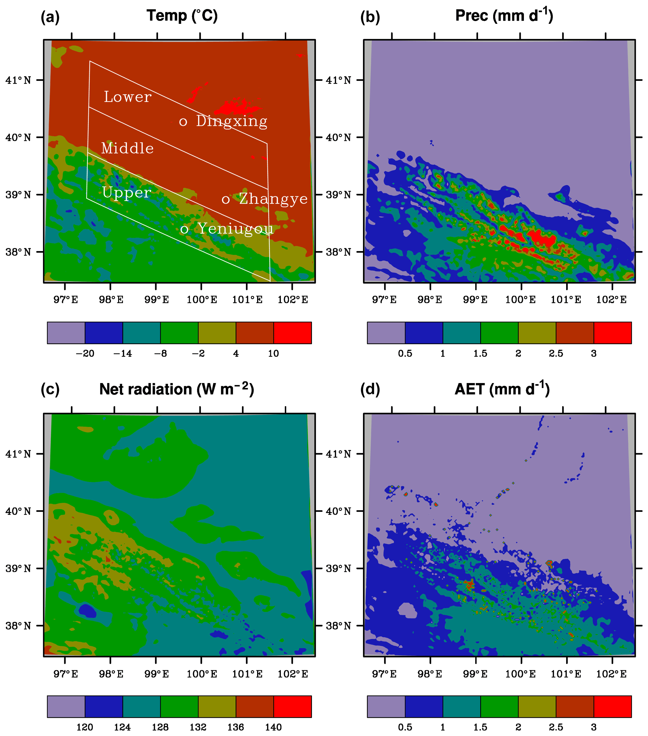
Figure 2Spatial distributions of the simulated air temperature (T, ∘C), precipitation (P, mm d−1), net radiation (NRAD, W m−2), and actual evapotranspiration (AET, mm d−1) averaged over 1980–2010. The Heihe River basins and weather stations are shown in (a).
An interesting feature is that both T and P in the middle basin are very close to their corresponding values in the lower basin but much different from those in the upper basin; the AET difference between the middle and upper basin reaches however is very small. As expected, the regional AET values averaged over the simulation period are higher in summer than in winter (Fig. 3). In the upper basin, for example, T increases from about −15 ∘C in winter to 10 ∘C in summer, P increased from about 0.25 to 4 mm d−1, and AET from about 0.25 to 2.5 mm d−1. Again, T and P are close between the middle and lower basin reaches in all seasons, and AET is close between the middle and upper basin reaches during winter and spring. While AET is close between the middle and lower basin reaches during summer and fall, the differences between the middle and upper basin reaches are much smaller than the differences in T or P. Net radiation has a seasonal cycle similar to that of temperature. The changing trends among the three basin reaches are the same between T and NRAD in spring and summer but opposite in winter and fall. The interannual variability of regional T and P is similar between the middle and lower basin reaches (Fig. 4). A few dry years (e.g., 1990, 2001, and 2008) and wet years (e.g., 1981, 1989, 2002, and 2007) can be found. The amplitude of variability is larger for P than T, especially in the upper basin. NRAD values have large interannual variability with little difference among the regions. The variability of AET is also similar between the lower and middle basin reaches, but it differs from that in the upper basin during some periods (e.g., around 1985). The differences in AET between the middle and upper basins are much smaller in the magnitude than those for the meteorological properties.
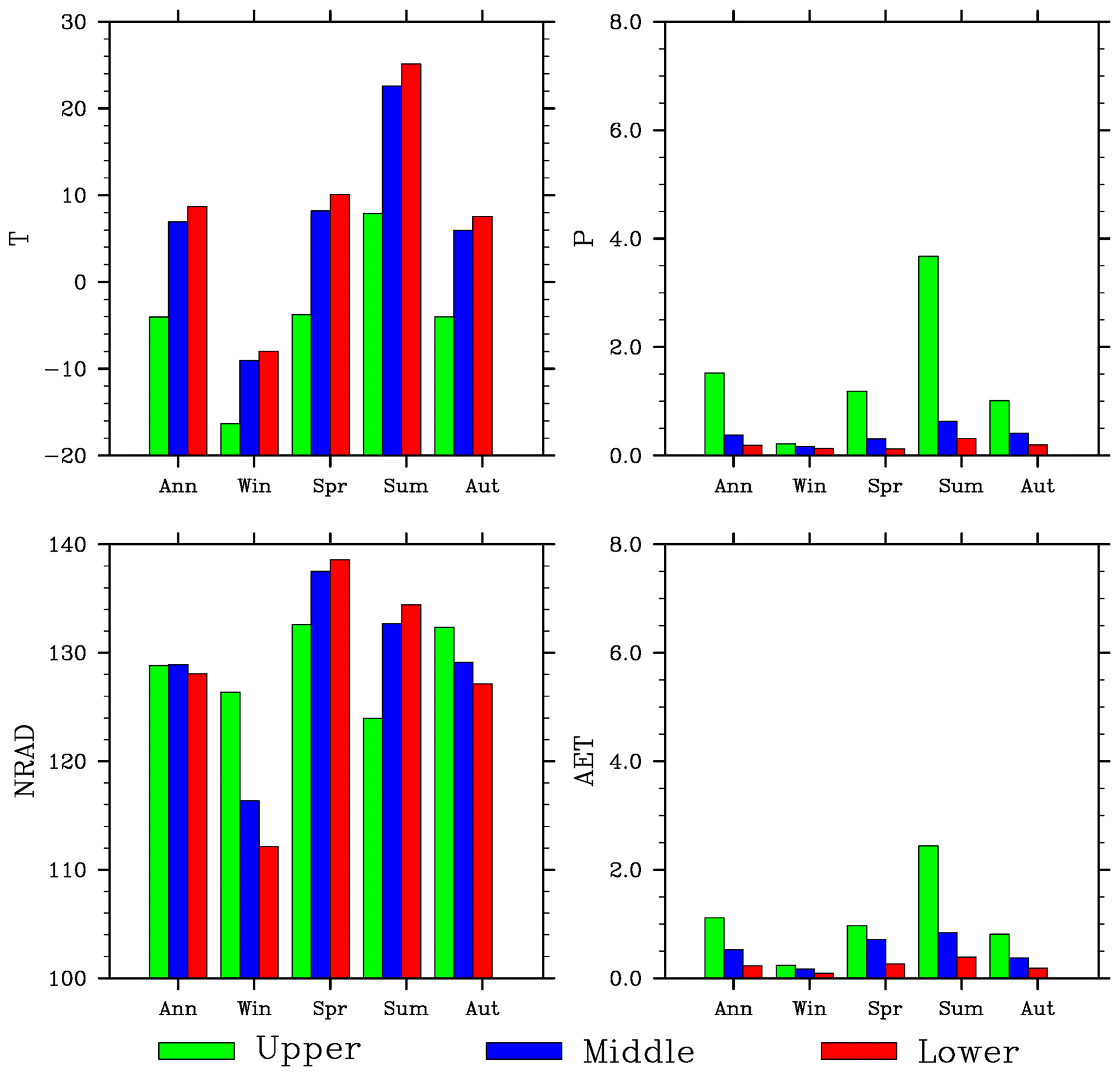
Figure 3Seasonal variations of the simulated air temperature (T, ∘C), precipitation (P, mm d−1), net radiation (NRAD, W m−2), and actual evapotranspiration (mm d−1) in three basin reaches averaged over 1980–2010.

Figure 4Interannual variations of the simulated air temperature (T, ∘C), precipitation (P, mm d−1), net radiation (NRAD, W m−2) and actual evapotranspiration (mm d−1), and observed air temperature (T, ∘C) and precipitation (P, mm d−1) in three basin reaches over 1980–2010.
The above features of close values and similar interannual variability in the simulated T and P between the middle and lower basin reaches are also seen in the observations (Fig. 4). The simulated T in all basin regions and P in the middle and lower basin reaches are close to the observed ones. However, the simulated P is about 0.4 mm d−1 higher (about 1.6 mm d−1 for simulation vs. 1.2 mm d−1 for observation). The weather site in the upper basin is located in a relatively flat and low valley, while the simulation grids have many points at high elevations where P is larger than at the valley locations. The SPI for the 12-month timescale also shows generally similar interannual variations over the analysis period between the simulated and observed precipitation in the three basins (Fig. 5). In the upper basin, for example, the observed wet spells occurred around 30, 50, 120, 230, 290, 340, and 360 months, while the dry spells occurred around 20, 30, 70, 100, 180, 200, 260, and 300 months. The simulation reproduces most of the wet and dry spells. However, the simulation is too wet during about 40–80 months and largely misses the dry events during 240–260 months.
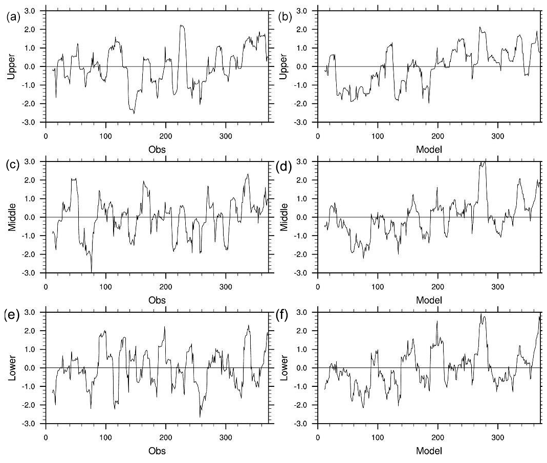
Figure 5The standardized precipitation index (SPI) for the 12-month timescale over the analysis period. The left panels (a, c, e) and right panels (b, d, f) are observation and simulation. From top to bottom are the upper (a, b), middle (c, d), and lower (e, f) basins. The horizontal number is the month from the beginning of the analysis period.
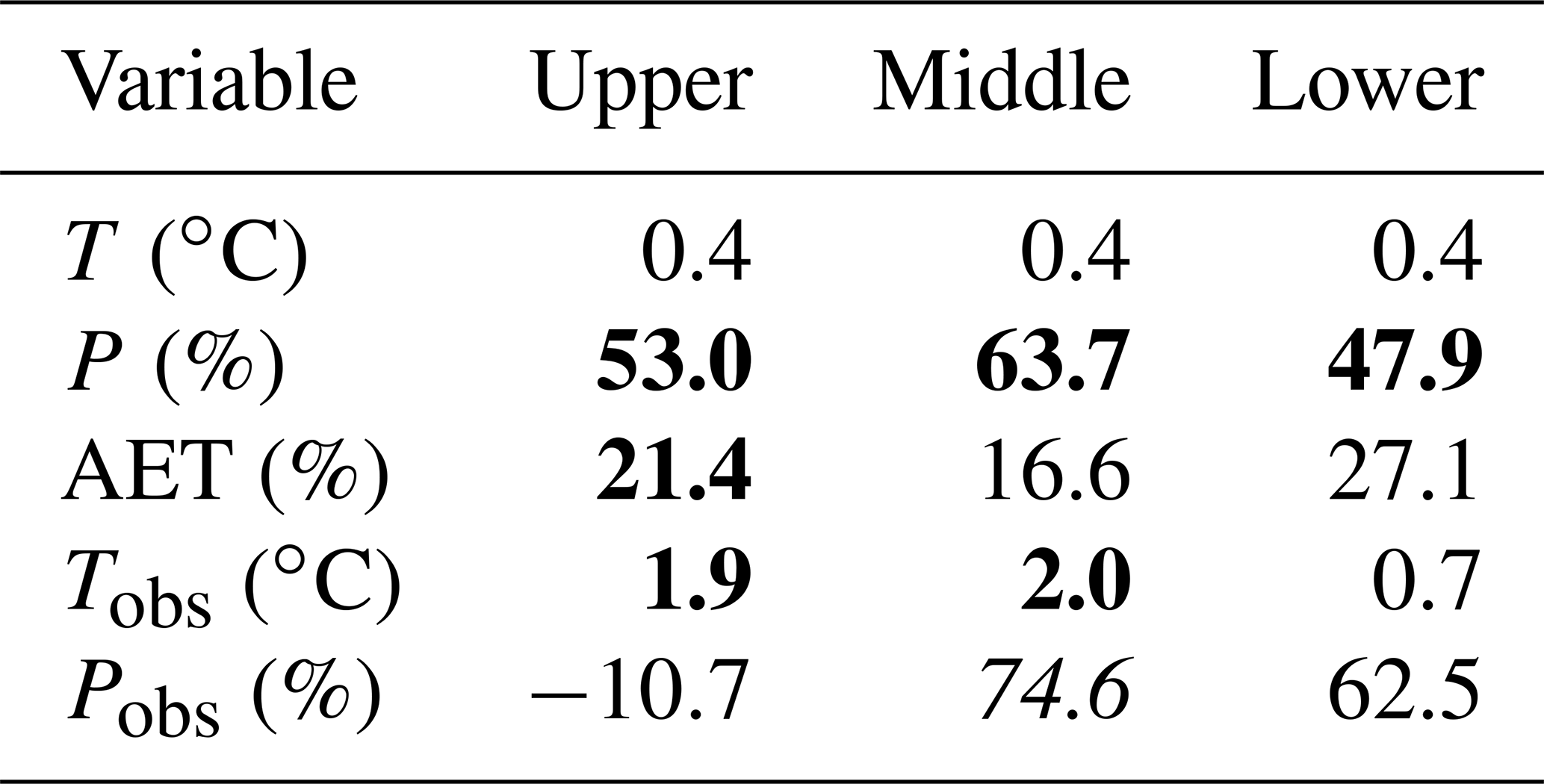
The simulated P increases around 50 % over the simulation period, which is statistically significant at p < 0.01 in all basin reaches (Table 2). The simulated AET also increases, but at a smaller degree of around 20 % and p < 0.01 only in the upper basin. The simulated T shows increasing trends, but they are insignificant in all reaches. The simulated P trends are close to the observed ones in the middle and lower basin reaches, but they are opposite to that in the upper basin. The simulated T underestimates the observed warming, which was about 2 ∘C at p < 0.01.
Table 2Mann–Kendall trends from 1980 to 2010 of the simulated temperature (T), precipitation (P), actual evapotranspiration (AET) and observed temperature (Tobs), and precipitation (Pobs). The bold and italic numbers are significant at p < 0.01 and p < 0.05, respectively.
3.2 Spatial patterns of aridity indices
PET calculated using the Penman–Monteith method is mostly 1.7–2.25 mm d−1 in the upper basin (Fig. 6). It increases to above 3 mm d−1 in the middle and lower basins. There is little difference between the two regions. The meteorological aridity index, AI, shows a similar pattern but opposite gradient (Fig. 6). It mostly has a humid climate in the upper basin but becomes mainly arid climate in two other basin regions. The hydrological aridity index, ESI, has the same gradient as AI, but with a different spatial pattern (Fig. 6). It also mostly has a humid climate in the upper basin and arid climate in the lower basin. However, it is largely semiarid climate in the middle basin. P and AET are the highest in the upper basin and the lowest in the lower basin, while T and PET have an opposite seasonal cycle. This explains why AI and ESI are larger in the upper basin than the middle or lower basin. PET calculated using the Hamon method has the same pattern as the one using the Penman–Monteith method, but with smaller magnitude (Fig. 7). PET is mostly about 1 mm d−1 in the upper basin and increases to about 1.5–1.75 mm d−1 in the middle basin and further to 1.75–2.25 mm d−1 in the lower basin.
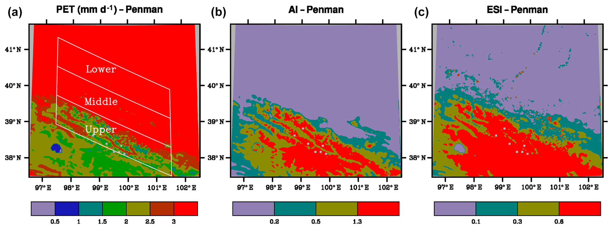
Figure 6Spatial distributions of potential evaporation (PET, mm d−1), aridity index (AI) and evaporative stress index (ESI) with PET estimated using the Penman–Monteith method. Averaged over 1980–2010. The Heihe River basins are shown in panel (a). The color bars from left to right for AI and ESI are arid, semiarid, semihumid and humid climate.
The different spatial patterns between AI and ESI seen above are also found for the Homan method. AI is mostly above 0.6 in the upper basin (Fig. 7). It is below 0.2 in the middle and lower basins without apparent differences between the two regions. In contrast, while ESI remains large with values of mostly above 0.9 in the upper basin and low values of below 0.2 in the lower basin, the values in many areas of the middle basin are 0.4–0.9, which are much different from those in the lower basin (Fig. 7).
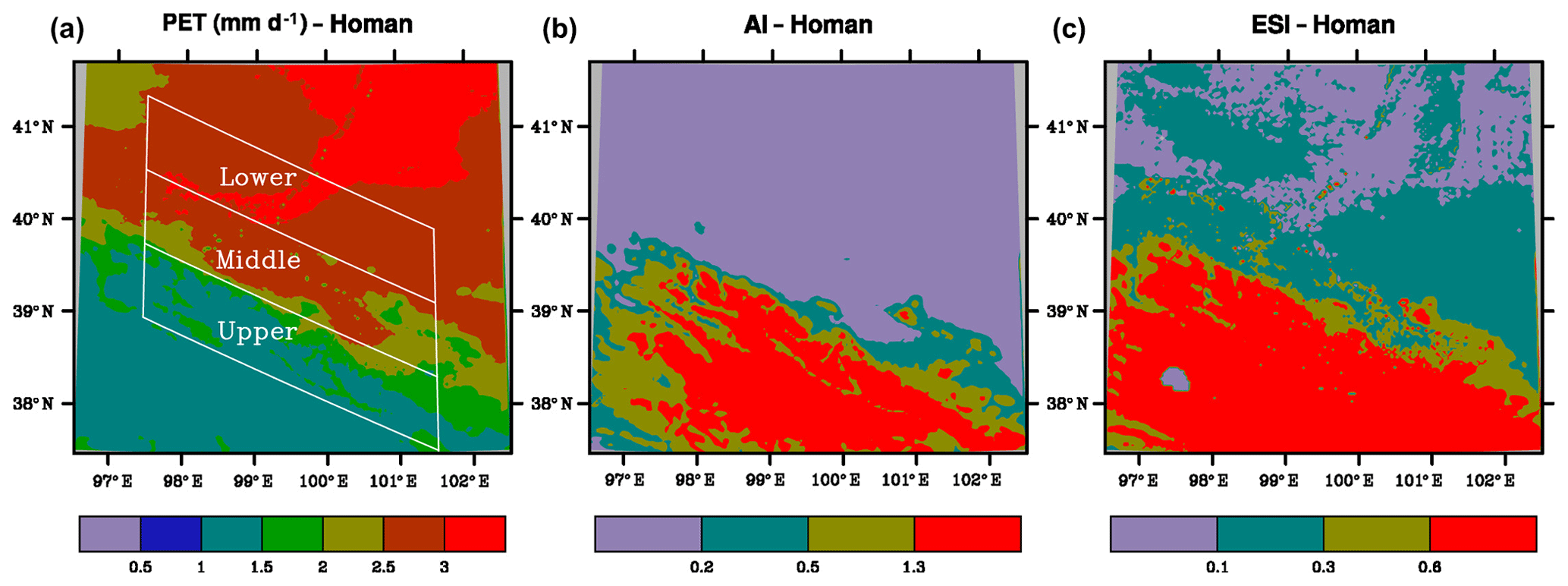
Figure 7Spatial distributions of potential evaporation (mm d−1), aridity index and evaporative stress index with PET estimated using the Hamon method. Averaged over 1980–2010. The Heihe River basins are shown in panel (a). The color bars from left to right for AI and ESI are arid, semiarid, semihumid and humid climate.
3.3 Climate classification
The annual PET averages over 1980–2010 calculated using the Penman method are 2.12, 3.91, and 4.76 (Table 3 and Fig. 8). The corresponding AI values are about 0.9, 0.12, and 0.04, falling into semihumid, arid, and arid climate. The corresponding ESI values are 0.63, 0.22, and 0.07, falling into humid, semiarid, and arid climate. The annual PET values averaged over 1980–2010 calculated using the Homan method are 1.25, 2.33, and 2.65 mm d−1 for the upper, middle, and lower basin reaches. The corresponding AI values are about 1.3, 0.18, and 0.07, falling into humid, arid, and arid climate. The corresponding ESI values are 0.78, 0.31, and 0.13, falling into humid, semihumid, and semiarid climate. The averages of PET or each of the aridity indices are statistically significant (p < 0.01) between any two regions of the Heihe River Basin.
Table 3Regional average (AVE), standard deviation (SD), and coefficient of variation (CV) for potential evapotranspiration (PET, mm d−1), aridity index (AI), and evaporative stress index (ESI). A, SA, SH, and H represent arid, semiarid, semihumid, and humid climate, respectively.
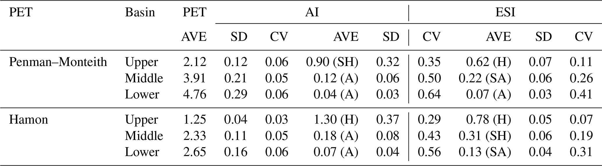
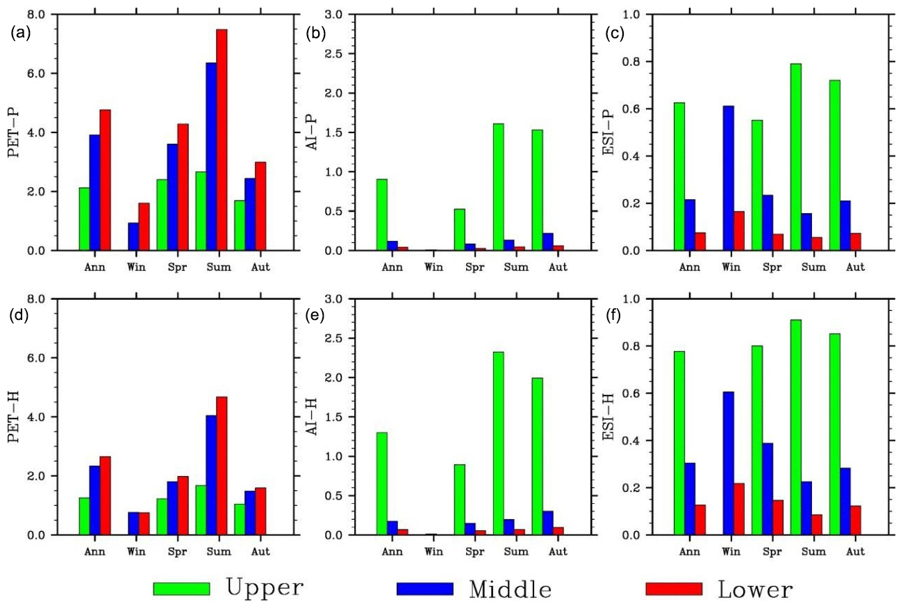
Figure 8Seasonal variations of the simulated potential evapotranspiration (mm d−1), aridity index, and evaporative stress index (from left to right). Panels (a)–(c) and (d)–(f) are for the Penman–Monteith and Hamon method, respectively.
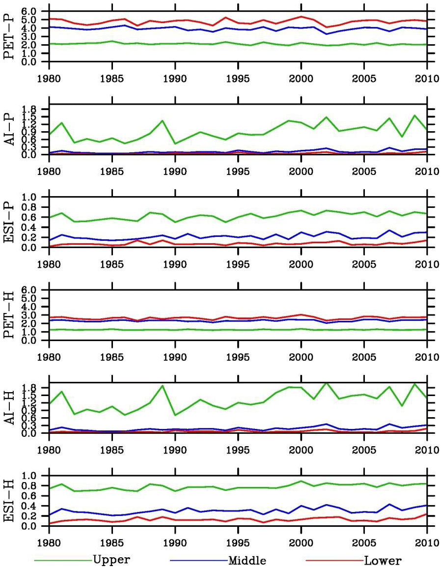
Figure 9Interannual variations of potential evapotranspiration (mm d−1), aridity index, and evaporative stress index. P and H indicate the Penman–Monteith and Hamon method, respectively.
Thus, the climate across the HRB classified using AI has two types: (i) semihumid (the Penman method for PET) or humid (the Homan method) in the upper basin and (ii) arid in both middle and lower basin reaches. In contrast, the climate classified using ESI has three types: (i) humid in the upper basin, (ii) semiarid (the Penman method) or semihumid (the Homan method) in the middle basin, and (iii) arid (the Penman method) or semiarid (the Homan method) in the lower basin. This indicates that only the hydrological aridity index is able to identify the transition climate zone in the middle basin. The difference between AI and ESI in classifying climate is related to the similar feature with the meteorological variables. Annual P is 555 mm in the upper basin, which is substantially different from 69–139 mm in the middle and lower basins. The mean T is −4.0 ∘C in the upper basin, which is well below 6.9–8.7 ∘C in the middle and lower basin reaches. The corresponding PET values fall into two groups, 299 mm in the upper basin and 672–767 mm in the middle and lower basin reaches. This explains why the AI falls into two groups. In contrast, AET is 226, 161, and 80 mm, which is substantially different not only between the middle and upper reaches but also between the middle and lower reaches. This explains why the ESI falls into three groups.
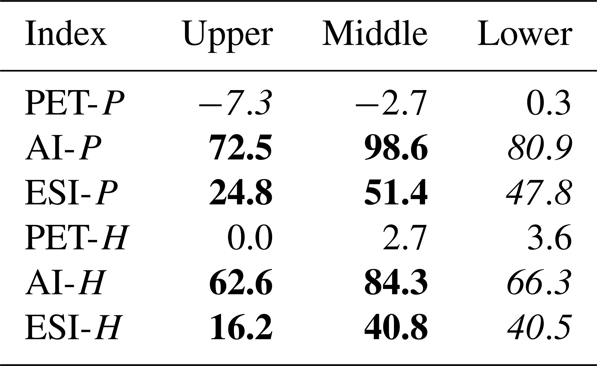
Table 4Mann–Kendall trends from 1980 to 2010 of potential evapotranspiration, aridity index, and evaporative stress index (in %). P(H) indicates the Penman–Monteith (Hamon) method. The bold and italic numbers are significant at p < 0.01 and p < 0.05.
3.4 Temporal variations of aridity indices
3.4.1 Seasonal cycle
For the Penman–Monteith method, PET is the highest in summer and smallest in winter (Fig. 8). Note that winter PET in the upper basin is not shown because T is below zero on too many days. The amplitude in the middle basin is close to that in the lower basin but much larger than that in the upper basin. Different from the upper basin where AI and ESI are also the largest in summer, AI is the largest in fall, while ESI is the largest in winter in the middle basin (as well as lower basin). The seasonal variations of PET, AI, and ESI estimated using the Homan method are similar to those using the Penman method.
The seasonal AI and ESI cycles are related to those of the meteorological and hydrological conditions. T, P and AET (Fig. 3), and PET (Fig. 8) all increase from winter to summer. In the upper basin, the increases in P and AET from spring/fall to summer are larger than the corresponding increases in PET, leading to larger AI and ESI values in summer. In the middle as well as lower basin, however, PET increases substantially from spring/fall, leading to a smaller AI and ESI in summer than in spring/fall.
3.4.2 Interannual variability
PET in the middle basin calculated using the Penman–Monteith method shows similar interannual variability over the period of 1980–2010 to that in the lower basin but much different from that in the upper basin (Fig. 9). The standard deviation (SD) increases from the upper basin (0.12) to the middle basin (0.21) and to the lower basin (0.29) (Table 2). The coefficient of variation (CV) (the ratio of the standard deviation to the average), a statistical property often used to measure relative variability intensity, however, is comparable among the reaches. The SD values of both AI and ESI decrease from the upper basin to the middle basin and to the lower basin. However, the SD of AI (ESI) in the middle basin is much closer to that in the lower (upper) basin. The CV values have an opposite gradient to SD, increasing from the upper basin to the middle basin and to the lower basin. In addition, CV differs mainly not between the basin reaches but between aridity indices: AI is larger than ESI.
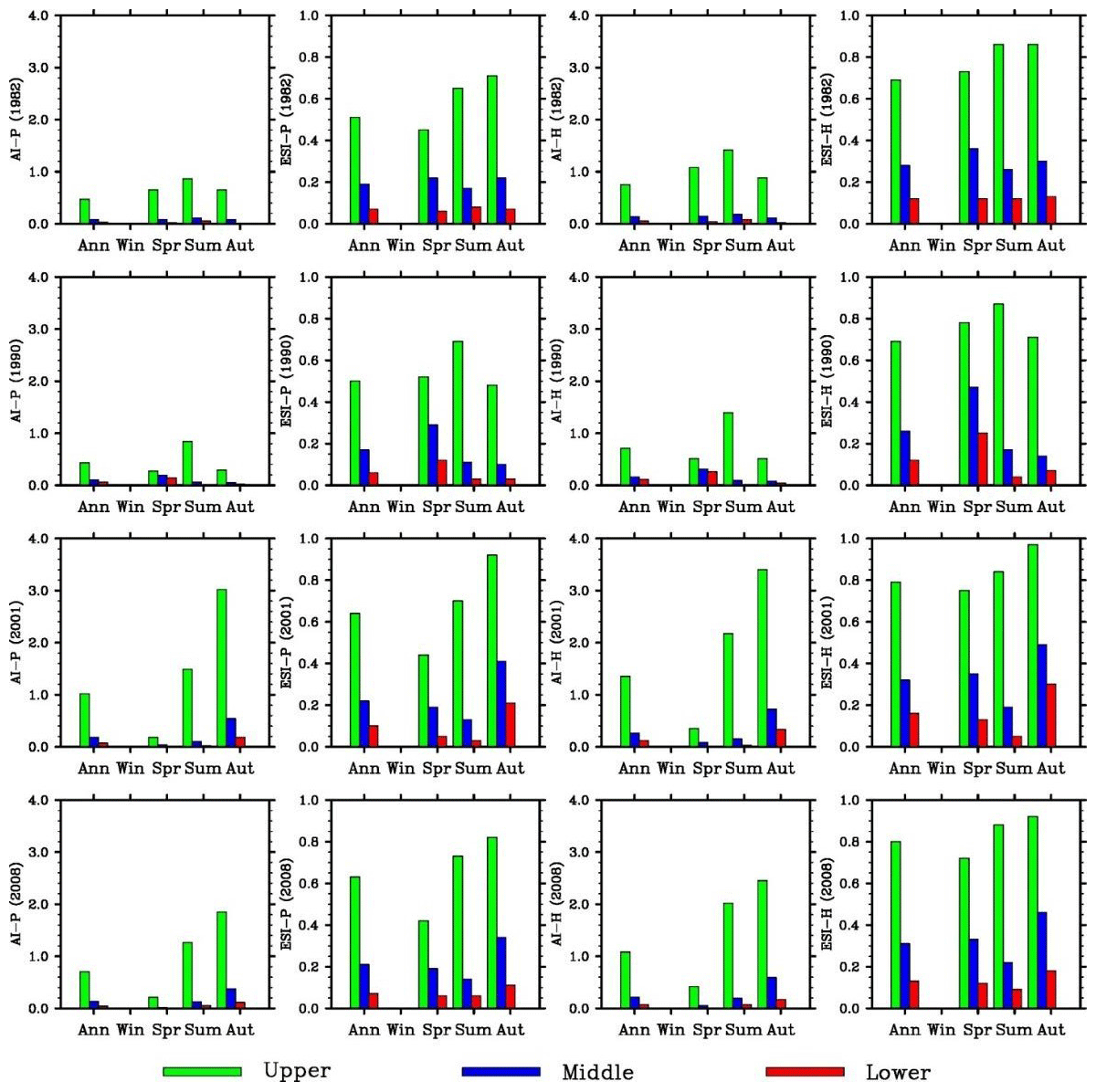
Figure 10Seasonal variations of the simulated aridity index and evaporative stress index using the Penman–Monteith and Hamon methods (left to right) for the dry years of 1982, 1990, 2001, and 2008 (from top to bottom).
3.4.3 Long-term trends
PET shows no clear trends over the simulation period (Table 4). In contrast, aridity indices increased dramatically, by 60 % or more for AI and 15 %–50 % for ESI. The trends are significant at p < 0.01 in the upper and middle basin reaches and p < 0.05 in the lower basin. The results indicate a lower dryness condition in the HRB, which is more remarkable in the middle than upper basin and in the meteorological than hydrological aridity index. Increase in precipitation is a major contributor.
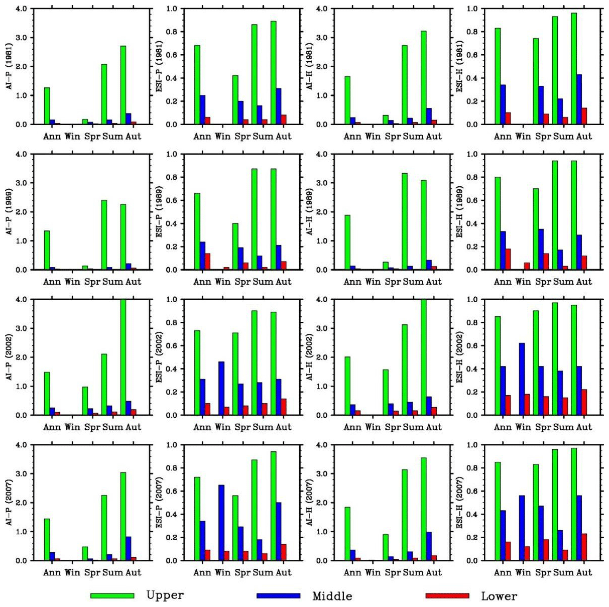
Figure 11Seasonal variations of the simulated aridity index and evaporative stress index using the Penman–Monteith and Hamon methods (left to right) for the wet years of 1981, 1989, 2002, and 2007 (from top to bottom).
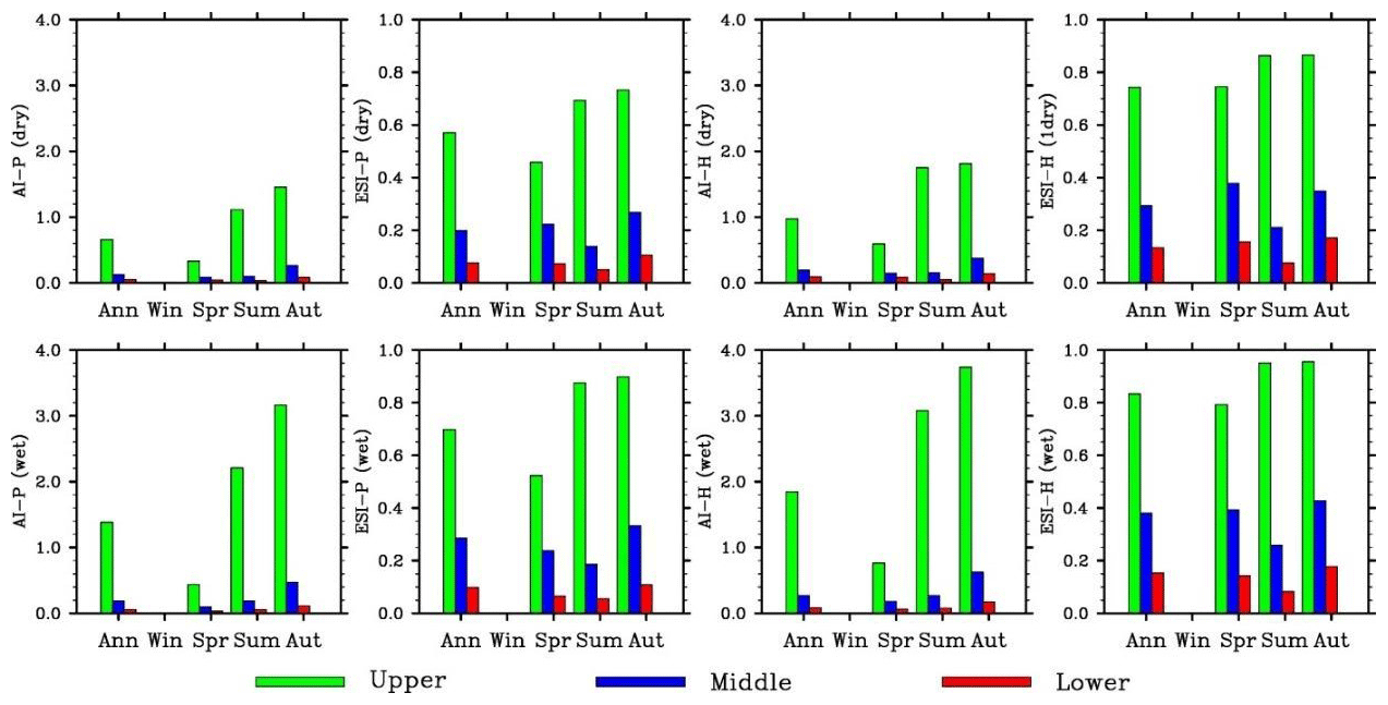
Figure 12Seasonal variations of the simulated aridity index and evaporative stress index using the Penman–Monteith and Hamon methods (left to right) for averages over the dry years of 1982, 1990, 2001, 2008 (top) and (bottom).
3.5 Extreme events
The aridity indices for four simulated dry years (1982, 1990, 2001, and 2008) and four wet years (1981, 1989, 2002, and 2007) (Figs. 10–11) and the averages over the dry or wet years (Fig. 12) were analyzed. The annual AI values using the Penman–Monteith method are 0.4–0.5 for the first two dry years and 0.7–1.0 for the last two years in the upper valley (Fig. 12). The average over the four years is about 0.65. In comparison, the average is about 0.9 over 1980–2010 and 1.4 over the four wet years. The values are very small in spring (except in 1982) and occasionally in fall (1990). The annual AI values in the middle and lower basin reaches are below 0.2 for individual dry years and the average. The small values are found for individual seasons except the falls of the last two years in the middle basin. In compassion, the annual values are 0.4 or above in three falls of the four wet years.
The annual ESI values using the Penman–Monteith method are 0.5 or larger in the upper valley. The average over the four years is nearly 0.6. In comparison, the average is about 0.62 over 1980–2010 and 0.7 over the four wet years. The values are comparable from spring to fall, though relatively smaller in spring. This is different from AI. The annual ESI values are about 0.2 in the middle and below 0.1 in the lower basin for individual dry years and the average. Thus, the values are apparently different between the middle and lower basin reaches. This is another difference from AI. The lowest values mostly occur in summer in both basin reaches. In compassion, the annual values are 0.25–0.35 in the middle basin and 0.1 or larger in three of the four wet years in the lower basin.
The same results can be found for the Hamon method. In the upper basin, AI is substantially smaller than normal, especially in spring, while ESI does not change much from normal and between seasons. In the middle and lower basin reaches, AI does not change much from normal and wet events (small in all cases), while ESI is much smaller than wet events and different between the two basin reaches, though AI and ESI values are slightly larger. The results suggest that ESI is more representative of extreme dry conditions in the middle basin but less sensitive to aridity in the upper basin.
4.1 Support of the integrated water–ecosystem–economy study in the HRB
The HRB is a typical inland river basin with a strong contrast in topography, landscape, climate, and human activities from the headwater to end point along its drainage system. Comprehensive monitoring, modeling, and data manipulation studies have been conducted for several decades to understand the hydrological and ecological processes and interactions in the HRB (Cheng et al., 2014). The middle HRB is a special region with dynamic land cover and use changes due to human activity. Different from the upper HRB regions where climate change has been the controlling factor for hydrological and ecological processes, surface water condition is extremely important in the middle HRB where irrigated farmland is the largest land use and natural oases have been gradually replaced by artificial oases (Li et al., 2001; Cheng et al., 2014). According to our study, the hydrological ESI should be a better indictor than the meteorological AI for water supply and demand conditions in the middle HRB. Zhang et al. (2015) found that the streamflow from the upper to middle HRB has risen due to climate change, but the streamflow from middle to lower HRB has decreased. They attributed this reduction to increasing water consumption by human activities in the middle HRB. Our study indicates a lower dryness trend in the middle HRB and therefore supports the analysis that climate change was not a major factor for the reduction. Sun et al. (2015) found an increasing trend in vegetation growth in the middle HRB and attributed it to irrigation. Our study shows a lower drying trend in this region, suggesting that more net water was another contributor to the increasing vegetation growth.
4.2 Importance of land-surface processes
The water shortage and frequent droughts are the biggest environmental threat to the ecosystems and human activities in the HRB as well as all of northwestern China. This comparison study provides evidence for the importance of water and energy interactions between land process and the atmosphere and between upstream and downstream in determining climate types in an arid climate. Because the ESI values are related to AET that is controlled by land-surface properties and management practices (e.g., rainfall-fed crops vs. irrigated crops and natural wetlands vs. cultivated drained croplands), our results suggest the land-surface processes play an important role in affecting aridity conditions. The landscape in the HRB, especially its transition zone, has changed remarkably over the past several decades due to urbanization, farming, and grazing activities (Hu et al., 2015). The irrigation may have caused the lower basin more water stress (higher ESI than AI) since stream water from the Heihe River is intercepted and rivers go dry downstream. The ESI should reflect this change since it is calculated partially based on the land-surface hydrological conditions. Urbanization, farming, and grazing would reduce vegetation coverage. This would further reduce evapotranspiration and increase runoff. Irrigation would play opposite roles. The RIEMS model uses the Biosphere and Atmosphere Transfer Scheme (BATS) (Dickinson and Henderson-Sellers, 1993) to simulate the land-surface hydrological processes. The vegetation and soil properties measured in the HRB in 2000 were used to replace the universal BATS specifications, which improved precipitation simulation (Xiong and Yan, 2013). However, the above disturbances over time were not included in the simulation that provided the data for this study. Numerical experiments with this model are needed to provide quantitative evidence for the hydrological effects of the disturbances.
4.3 Role in moderating climate
The magnitude of AI (ESI) interannual variability in the middle basin is (is not) very close to that in the lower basin, which is additional evidence for the unique capacity of ESI to separate the climate zones between the middle and lower basin reaches. The magnitude of the relative interannual variability differs mainly between AI and ESI and is larger with AI. In addition, both AI and ESI in the HRB decreased dramatically from 1980 to 2010, with AI decreasing at a greater rate. Thus, the aridity conditions described using ESI are less variable, suggesting the role of local hydrological processes in moderating extreme climate events.
4.4 Future trends
One of the hydrological consequences from the projected climate change due to the greenhouse gas increase is more frequent and intense droughts in watersheds of dry regions. In the Colorado River Basin, global warming may lead to substantial water supply shortages (McCabe and Wolock, 2007), and the climate models projected considerably more drought activities in the 21st century (Cayan et al., 2010). In the HRB, the climate of the upper HRB will likely become warmer and wetter in the near future (Zhang et al., 2016), consistent with the historical records. Correspondingly the basin-wide evapotranspiration, snowmelt, and runoff are projected to increase over the same period. Many aridity indices, including the AI, have been used to project future aridity trends (Paulo et al., 2012). However, most of the recent ESI studies are based on historical remote sensing for monitoring short-term drought development, which limits the application of this index to climate change impact research. Due to the unique ability of the ESI to identify the transition climate zone as shown in this study, it would be valuable to explore its potential for future aridity projection study and compare with that of the AI.
4.5 Uncertainty and future research
The regional climate simulation which generated data for this analysis has many uncertainties (Xiong and Yan, 2013). One of the contributing factors is the very limited number of meteorological, hydrological, and ecological measurement sites. A large-scale, multiple-year field experiment project has been conducted in the HRB, which has generated extensive datasets (Wang et al., 2014). These data are being used to improve the regional climate modeling, which will in turn generate new high-resolution data for further aridity analysis. Furthermore, the regional climate modeling has been expanded into the middle 21st century, providing data for calculating the aridity indices and comparing their future trends. Comparisons of other meteorological and hydrological aridity indices are also a future research issue.
This study has found that the ESI climate classification agrees with the Köppen climate classification (Peel et al., 2007). By using ESI, we found that the climate types are different among the upper, middle, and lower HRB. In contrast, there is no difference between the middle and lower HRB regions when the AI is used. The comparison results from this study therefore suggest that only ESI is able to identify a transition climate zone between the relatively humid climate in the mountains and the arid climate in the Gobi desert region. We conclude that the hydrological aridity index ESI is a better index than the meteorological aridity index AI for climate classification in the HRB with a complex topography and land cover. Selection of the most appropriate aridity index facilitates climate characterization and assessment, risk mitigation, and water resource management in the arid region.
The regional climate modeling data and weather station observational data used in this study are not stored in a publicly accessible database due to their very large size. They are available upon request from the corresponding author.
YL performed the calculations and wrote the manuscript; LH and GS led this research; ZX conducted the regional climate modeling; and DZ, CP, and PL participated in discussion.
The authors declare that they have no conflict of interest.
We thank the reviewers for their valuable and insightful comments and suggestions.
This research has been supported by the National Natural Science Foundation of China (grant no. 91425301).
This paper was edited by Kai Schröter and reviewed by three anonymous referees.
Allen, R. G., Pereira, L. S., Raes, D., and Smith, M.: “Crop evapotranspiration: guidelines for computing crop water requirements.” Irrigation and Drainage Paper No. 56, Food and Agriculture Organization of the United Nations, Rome, Italy, 1998.
Anderson, M. C., Hain, C. R., Wardlow, B., Mecikalski, J. R., and Kustas, W. P.: Evaluation of drought indices based on thermal remote sensing of evapotranspiration over the continental U.S, J. Climate, 24, 2025–2044, 2011.
Anderson, M. C., Zolin, C. A., Sentelhas, P. C., Hain, C. R., Semmens, K., Yilmaz, M. T., Gao, F., Otkin, J. A., and Tetrault, R.: The Evaporative Stress Index as an indicator of agricultural drought in Brazil: An assessment based on crop yield impacts, Remote Sens. Environ., 174, 82–99, https://doi.org/10.1016/j.rse.2015.11.034, 2016.
Budyko, M. I.: Climate and Life, Academic, San Diego, CA, 508 pp., 1974.
Cayan, D. R., Das, T., Pierce, D. W., Barnett, T. P., Tyree, M., and Gershunov, A.: Future dryness in the southwest US and the hydrology of the early 21st century drought, P. Natl. Acad. Sci. USA, 107, 271–21, 2010.
Chen, Y., Zhang, D., Sun, Y., Liu, X., Wang, N., and Savenije, H.: Water demand management: A case study of the Heihe River Basin in China, Phys. Chem. Earth, 30, 408–419, https://doi.org/10.1016/j.pce.2005.06.019, 2005.
Cheng, G. D., Li, X., Zhao, W. Z., Xu, Z. M., Feng, Q., Xiao, S. C., and Xiao, H. L.: Integrated study of the water–ecosystem–economy in the Heihe River Basin, Nat. Sci. Rev., 1, 413–428, https://doi.org/10.1093/nsr/nwu017, 2014.
Choi, M., Jacobs, J. M., Anderson, M. C., and Bosch, D. D.: Evaluation of drought indices via remotely sensed data with hydrological variables, J. Hydrol., 476, 265–273, https://doi.org/10.1016/j.jhydrol.2012.10.042, 2013.
Dickinson, R. E. and Henderson-Sellers, A.: Biosphere-Atmosphere Transfer Scheme (BATS) Version as coupled to the NCAR Community Climate Model, NCAR Technical Report, NCAR/TN-387+STR, 1993.
Gao, B., Qin, Y., Wang, Y. H., Yang, D., and Zheng, Y.: Modeling Ecohydrological Processes and Spatial Patterns in the Upper Heihe Basin in China, Forests, 7, https://doi.org/10.3390/f7010010, 2016.
Guttman, N. B.: Accepting the standardized precipitation index: a calculation algorithm, JAWRA J. Am. Water Resour. Assoc., 35, 311–322, https://doi.org/10.1111/j.1752-1688.1999.tb03592.x, 1999.
Hamon, W. R.: Computation of direct runoff amounts from storm rainfall. Intl. Assoc. Scientific Hydrol. Publ., 63, 52–62, 1963.
Hu, X., Lu, L., Li, X., Wang, J., and Guo, M.: Land use/cover change in the middle reaches of the Heihe River Basin over 2000–2011 and its implications for sustainable water resource management, PLoS ONE, 10, e0128960, https://doi.org/10.1371/journal.pone.0128960, 2015.
Huschke, R. E.: Glossary of Meteorology, American Meteorological Society, Boston, 1959.
Keetch, J. J. and Byram, G. M.: A drought index for forest fire control, USDA Forest Service Research Paper No. SE38, pp. 1–32, 1968.
Li, J.: Multivariate Frequencies and Spatial Analysis of Drought Events Based on Archimedean Copulas Functio, Northwest University of Science and Technology, 2012.
Li, X., Lu, L, Cheng, G. D., and Xiao, H. L.: Quantifying landscape structure of the Heihe River Basin, north-west China using FRAGSTATS, J. Arid Environ., 48, 521–535, https://doi.org/10.1006/jare.2000.0715, 2001.
Maliva, R. and Missimer, T.: Arid Lands Water Evaluation and Management, available at: https://www.springer.com/us/book/9783642291036 (last access: 8 October 2019), 21–39, 2012.
McCabe, G. J. and Wolock, D. M.: Warming may create substantial water supply shortages in the Colorado River basin, Geophys. Res. Lett., 34, L22708, https://doi.org/10.1029/2007GL031764, 2007.
McKee, T. B., Doesken, N. J., and Kleist, J.: The Relationship of Drought Frequency and Duration to Time Scales, Proceedings of the Eighth Conference on Applied Climatology, American Meteorological Society, Boston, 17–22 January 1993, Anaheim, 179–184, 1993.
Nalbantis, I. and Tsakiris, G.: Assessment of hydrological drought revisited Water Resour. Manag., 23, 881–97, 2009.
Narasimhan, B. and Srinivasan, R.: Development and evaluation of soil moisture deficit index and evapotranspiration deficit index for agricultural drought monitoring, Agricult. Forest Meteorol., 133, 69–88, 2005.
Otkin, J. A., Anderson, M. C., Hain, C. R., Mladenova, I. E., Basara, J. B., and Svoboda, M.: Examining rapid onset drought development using the thermal infrared based Evaporative Stress Index, J. Hydrometeorol., 14, 1057–1074, 2013.
Palmer, W. C.: Meteorological drought, U.S. Research Paper No. 45, US Weather Bureau, Washington, DC, available at: https://www.ncdc.noaa.gov/temp-and-precip/drought/docs/palmer.pdf (last access: 8 October 2019), 1965.
Paulo, A. A., Rosa, R. D., and Pereira, L. S.: Climate trends and behaviour of drought indices based on precipitation and evapotranspiration in Portugal, Nat. Hazards Earth Syst. Sci., 12, 1481–1491, https://doi.org/10.5194/nhess-12-1481-2012, 2012.
Peel, M. C., Finlayson, B. L., and McMahon, T. A.: Updated world map of the Köppen-Geiger climate classification, Hydrol. Earth Syst. Sci., 11, 1633–1644, https://doi.org/10.5194/hess-11-1633-2007, 2007.
Ponce, V. M., Pandey, R. P., and Ercan, S.: Characterization of drought across climatic spectrum, J. Hydrol. Eng., 5, 222–2245, 2000.
Ren, Z., Lu, Y., and Yang, D.: Drought and flood disasters and rebuilding of precipitation sequence in Heihe River basin in the past 2000 years, J. Arid Land Resour. Environ., 24, 91–95, 2010.
Shafer, B. A. and Dezman, L.E.: Development of a Surface Water Supply Index (SWSI) to assess the severity of drought conditions in snowpack runoff areas. In Proceedings of the Western Snow Conference, Colorado State Univ., Fort Collins, CO. 164–175, 1982.
Shukla, S. and Wood, A. W.: Use of a standardized runoff index for characterizing hydrologic drought, Geophys. Res. Lett., 35, L02405, https://doi.org/10.1029/2007GL032487, 2008.
Sun, W., Song, H., Yao, X., Ishidaira, H., and Xu, Z.: Changes in remotely sensed vegetation growth trend in the Heihe basin of arid northwestern China, PLoS ONE, 10, e0135376, https://doi.org/10.1371/journal.pone.0135376, 2015.
Svoboda, M., LeComte, D., Hayes, M., Heim, R., Gleason, K., Angel, J., Rippey, B., Tinker, R., Palecki, M., Stooksbury, D., Miskus, D., and Stephin, S.: The Drought Monitor, B. Am. Meteorol. Soc., 83, 1181–1190, 2002.
Wang, L. X., Wang, S. G., and Ran, Y. H.: Data sharing and data set application of watershed allied telemetry experimental research, IEEE Geoscience Remote Sens. Lett., 11, 2020–2024, https://doi.org/10.1109/LGRS.2014.2319301, 2014.
Wilhite, D. A. and Glantz, M. H.: Understanding the drought phenomenon: The role of definitions, Water Int., 10, 111–120, 1985.
Woodhouse, C. A., Meko, D. M., MacDonald, G. M., Stahle, D. W., and Cook, E. R.: A 1200-year perspective of 21st century drought in southwestern North America, P. Natl. Acad. Sci. USA, 107, 21283–21288, 2010.
Xiong, Z. and Yan, X. D.: Building a high-resolution regional climate model for the Heihe River Basin and simulating precipitation over this region, Chin. Sci. Bull, 58, 4670–4678, 2013.
Yang, D. W., Gao, B., Jiao, Y., Lei, H. M., Zhang, Y. L., Yang, H. B., and Cong, Z. T.: A distributed scheme developed for eco-hydrological modeling in the upper Heihe River, Sci. China Earth Sci., 58, 36–45, https://doi.org/10.1007/s11430-014-5029-7, 2015.
Yang, G. H.: Agricultural Resources and Classification, China Agricultural Press, Beijing, China, 286 pp., 2007.
Yao, A. Y. M.: Agricultural potential estimated from the ratio of actual to potential evapotranspiration, Agricult. Meteorol., 13, 405–417, https://doi.org/10.1016/0002-1571(74)90081-8, 1974.
Zargar, A., Sadiq, R., Naser, B., and Khan, F. I.: A review of drought indices, Environ. Rev., 19, 333–349, 2011.
Zhang, A. J., Zheng, C. M., Wang, S., and Yao, Y. Y.: Analysis of streamflow variations in the Heihe River Basin, northwest China: Trends, abrupt changes, driving factors and ecological influences, J. Hydrol., 3, 106–124, 2015.
Zhang, A. J., Liu, W. B., Yin, Z. L., Fu, G. B., and Zheng, C. M.: How will climate change affect the water availability in the Heihe River Basin, Northwest China?, J. Hydrometeorol., 1517–1542, https://doi.org/10.1175/JHM-D-15-0058.1, 2016.