the Creative Commons Attribution 4.0 License.
the Creative Commons Attribution 4.0 License.
 | 02 Sep 2019
Coastline evolution based on statistical analysis and modeling
Elvira Armenio
Francesca De Serio
Michele Mossa
Antonio F. Petrillo
Wind, waves, tides, sediment supply, changes in relative sea level and human activities strongly affect shorelines, which constantly move in response to these processes, over a variety of timescales. Thus, the implementation of sound coastal zone management strategies needs reliable information on erosion and/or deposition processes. To suggest a feasible way to provide this information is the main reason for this work. A chain approach is proposed here, tested on a vulnerable coastal site located along southern Italy, and based on the joint analysis of field data, statistical tools and numerical modeling. Firstly, the coastline morphology has been examined through interannual field data, such as aerial photographs, plane-bathymetric surveys and seabed characterization. After this, rates of shoreline changes have been quantified with a specific GIS tool. The correlations among the historical positions of the shoreline have been detected by statistical analysis and have been satisfactorily confirmed by numerical modeling, in terms of recurrent erosion–accretion area and beach rotation trends. Finally, based on field topographic, sediment, wave and wind data, the response of the beach through numerical simulation has been investigated in a forecasting perspective. The purpose of this study is to provide a feasible, general and replicable chain approach, which could help to thoroughly understand the dynamics of a coastal system, identify typical and recurrent erosion–accretion processes, and predict possible future trends, useful for planning of coastal activities.
- Article
(3706 KB) - Full-text XML
- BibTeX
- EndNote


Beachfront lands are the place where unique and fragile natural ecosystems evolve in equilibrium with the ever-changing forces of wind, waves and water levels. Even if highly vulnerable to natural hazards including marine inundation, floods, storm impacts, sea level rise and coastal erosion, these coastal areas are the site of intense residential and commercial development, thus being even more vulnerable. Shoreline evolution, characterized by erosion and deposition areas, has consequences on socioeconomic activities and ecosystems. Therefore their evolution and understanding represent a challenge to coastal communities, coastal infrastructures and adjacent estuarine environments (Cutter et al., 2008; Torresan et al., 2012; De Serio and Mossa, 2014, 2016; Samaras et al., 2016; De Padova et al., 2017; Armenio et al., 2017a, 2018).
Moreover, coastal environments are subject to continual adjustments towards a dynamic equilibrium, differently responding to fluvial/sea-dominated events. Thus, in a context of changing the climate, understanding processes connecting fluvial and coastal systems is of paramount importance (Termini, 2018). As observed by Bonaldo et al. (2019), one of the most striking difficulties when dealing with coastal morphological vulnerability is to harmonize information about different disciplines and coming from different sources into the description of physical processes occurring at different time and spatial scales. To evaluate changes in coastal regions and recognize some key physical processes over different historical timescales (decade to century), data of shoreline geometry and position are basic indicators. A quantitative analysis of data of shoreline evolution at different timescales and with a fine spatial resolution is fundamental in establishing the processes driving erosion and accretion (De Serio at al., 2018; Elfrink et al., 1998; Katz and Mushkin, 2013; Thébaudeau et al., 2013; Oyedotun, 2014). Thus, various statistical methods of determining rates of shoreline change have been studied and applied (Dolan et al., 1991).
One of the simplest methods is the end-point rate (EPR) method, which estimates the distance of the shoreline movement rated by the time elapsed between the oldest and the most recent shoreline (Genz et al., 2006). Foster and Savage (1985) used the average of rates (AOR) method, which computes separate end-point rates for more than two combinations of shorelines. The linear regression rate-of-change (LRR) statistic has been used by fitting a least-squares regression line to all shoreline points for a transect (Dolan et al., 1977), thus deducing the rate as the slope of the line. An iterative linear regression fitting all possible combinations of shoreline points, leaving out one point in each iteration, has also been implemented, i.e., the jackknife (JK) method (Dolan et al., 1991). In addition to the above-written established methods, the weighted linear regression (WRL) method has also been used (Genz et al., 2006). In this case, more reliable data are given greater emphasis, or weight, defined as a function of the variance in the uncertainty of the measurement.
Questions arise about the appropriateness of linear models, considering that shorelines do not recede or accrete uniformly (Douglas and Crowell, 2000; Thieler and Danforth, 1994a, b). As an example, coastal embayments featured by a parabolic curve, which are representative of more than 50 % of the world's coastlines, are very dynamic environments where the shoreline position can fluctuate significantly due to processes such as beach rotation (Armenio et al., 2017b; Short and Trembanis, 2004; Blossier et al., 2015). This can be defined as the landward or seaward movement at one end of the beach accompanied by the reverse pattern at the other end (Bryan et al., 2013) and is often a consequence of maritime constructions (i.e., dikes, breakwaters) and variations in river sediment supply on flanking beaches. In the shorter term, changes in wave direction could also contribute to this marked shoreline readjustment.
Besides the statistical analysis of data, for the long-term shoreline evolution the use of analytical, morphodynamic and physical models has also been increasingly demanded (Deigaard et al., 1986a, b; Dean and Dalrymple, 2004; Davidson et al., 1991; Thomas and Frey, 2013). Nevertheless, coastal morphodynamic models require large computational resources and time and, consequently, they are scarcely suitable to the large spatial and temporal scales over which beaches evolve. Physical models are well suited to local analysis but are often prohibitive to be used for very large scales. This means that the increasing complexity of used models does not necessarily improve the predictions. Moreover, all models need to be calibrated and validated through sensitivity analyses, which are demanding for rich and complete sets of data (Armenio et al., 2017c, 2016).
In this work we aim to show that (i) the statistical analysis of data remains an accurate method to characterize shoreline changes, even if it disregards potential changes due to engineering activities or major climate change, (ii) the use of a simple one-line numerical model, based on the conservation of sand volume equation, is still satisfactory to evaluate shorelines changing, with the advantage of being feasibly applicable. Therefore, the present paper proposes a chain approach to detect information on the shoreline evolution, based on statistical analysis and one-line modeling (Fig. 1).
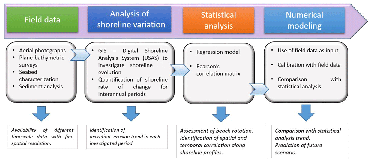
Firstly, field information and shoreline data have been analyzed to examine the past behavior of the coastal system and the effects of human activities on shoreline movement and rates of change. After this, GIS tools have been used for the quantification of shoreline rate of change for interannual periods.
A regression model and the Pearson's correlation matrix have been used to statistically investigate possible correlations of historical shoreline profiles. Finally, the numerical model LITPACK developed by the DHI – Danish Hydraulic Institute (DHI, 2016), implemented with field data, has been validated with hindcasting and used for a short-term shoreline prediction.
This approach has been applied to a target area located in southern Italy along the Adriatic Sea, characterized by a coastline 18 km long and described in Sect. 2. Section 3 illustrates the long period and the fine-resolution spatial data derived from the observations collected for this site. It also explains the principal features of the used GIS tool and LITPACK model. The quantitative analysis of shoreline changes in space and time is presented in Sect. 4, while Sect. 5 shows the results of the numerical simulation, in both hindcasting and forecasting terms. The presented results are site-specific but the used procedure is general, replicable and applicable to similar data sets.
The study area is in the southeastern coast of the Apulian region (Italy) along the Adriatic Sea, namely in the Gulf of Manfredonia. It extends from Margherita di Savoia town to Barletta town, with a total length of about 18 km (Fig. 2). The coast here is typically a low sandy beach with dunes, wetlands and salt marshes. At approximately 2 km off the coast, the depth is around 13 m. This sandy coast has originated over the years from the sediments supplied by several rivers, flowing into the gulf. The coast neighboring Margherita di Savoia is mainly due to the solid transport contribution of the most important river of the region, the Ofanto River, whose length and flow rate are respectively 134 km and 15 m3 s−1 (annual average).

Figure 2Study area with notation of Cell I–Cell III. Source © Google Earth.
In the last 2 centuries, both the rivers and the coastal area have experienced remarkable transformations, especially due to strong human activity, with consequent alternating erosion and deposition processes. In the early 1800s during some remediation works, river sediments were used to bury marshes and in canalization works, thus provoking a reduction in sediment supply from land and widespread coastal erosion. In the mid-1900s, several reservoirs and crossbars were constructed on the Ofanto River and its tributaries, to assure water supply for irrigation, industrial and drinking uses. Since 1960, the intense urbanization of the coastal zone has provoked critical local issues, further contributing to erosion phenomena. Probably the most perturbing cause in the coastal dynamics between the Ofanto's mouth and Manfredonia town (Fig. 2) was the construction of the port of Margherita di Savoia, started in 1952 and completed 40 years later. The prevailing direction of the solid longitudinal transport along the Apulian coast is from north to south. Intercepting the rich coastal flow of sediments, this structure has always had a great impact on the adjacent coast, altering the beach equilibrium and inducing over the years localized heavy erosion and accumulation, thus leading to a change in the coastal morphology from a linear to curved beach profile (Damiani et al., 2003).
This coastal sector is subjected to predominant NNW and SSE winds and the annual wave climate is characterized by a bimodal regime with a clear predominance of waves from N to NNE and E to ESE (Apulian Coastal Plan, 2012). The maximum significative wave height is in the range of 1–2 m, while the most frequent one is in the range of 0.5–1 m.
For the aim of the present work, the coastline in the study area has been divided into three parts with relatively homogeneous geomorphological change patterns, named Cell I, Cell II and Cell III (Fig. 2). They all have a curvy geometry. Cell I and Cell III are two concave beaches (i.e., curved towards the sea) and are separated by Cell II, which is convex (i.e., curved towards the inland). Cell I is delimited by the Margherita di Savoia port to the north and by the Ofanto River's mouth to the south. It has a length of about 6.0 km. Cell II extends from the Ofanto River's mouth up to a residential area called Fiumara, for a total length of about 1.5 km (Fig. 2). Its convex coastline is characterized by the alternation of sandy and rocky beaches, with breakwaters and riprap seawalls also placed to protect the beach. Cell III connects the Fiumara site with the Barletta port, with a total length of about 8.6 km of sandy beaches.
3.1 Availability of aerial and land data
To detect and quantify an erosion–accretion phenomenon, longtime observations are necessary for analyzing the evolution of the shoreline and thus to eliminate the influence of seasonal, episodic events such as individual storm surges and local sedimentary dynamics. For the present study, interannual field observations are adopted to map the historic coastline configurations. Shoreline positions have been derived from aerial photographs, digital orthophotos and global positioning system field surveys, acquired during a research activity carried out by the research unit of DICATECh (Polytechnic University of Bari) in recent years. As is well known, the idealized definition of shoreline is that it coincides with the physical interface of land and water, but this definition is in practice a challenge to apply. The most common shoreline detection technique applied to visibly discernible shoreline features is a manual visual interpretation, either in the field or from aerial photography (Boak and Turner, 2005). With aerial photography, the image has been corrected for distortions and then geo-referenced and adjusted to the correct scale; thus the shoreline has been digitized. In the field, a GPS has been used to digitize the visible shoreline feature in situ, as determined by the operator. Attention has been paid to ensure accurate digitization and a critical review of the source materials. Possible approximations could be due to difficulties in the interpretation of aerial photographs because of waves, swimmers and boats, or in geo-referencing aerial images because of wrong reference points. Consequently, we have assumed the gaps between two shorelines in the range ±3 m to be negligible (Chiaradia et al., 2008). This accuracy is important, considering that the calculated measures of change obtained by the Digital Shoreline Analysis System (DSAS) are only as reliable as the sampling and measurement accuracy associated with the source materials (Oyedotun, 2014). Data have been digitized and appropriately overlapped for comparison relative to the years 1992, 1997, 2006, 2008, 2011 and 2013. Closer to the shoreline, fine-resolution data assessed during a bathymetric survey performed in 2006 have been added. A plane-bathymetric survey and sediment analysis carried out in 2009 has also provided information on the nature of the seabed. A total of 15 onshore samples have been collected at five cross-shore beach profiles along the target area between depths of 1.73 and 6.12 m. They are mostly composed of sand with a mean diameter in the range of 1.67–2.21 mm (Apulian Coastal Plan, 2012).
3.2 GIS application
In recent years, the geographic information system (GIS) technology has been used to create high-quality maps and visualize and simplify large data. Specifically, to quantify the coastal evolution in the investigated period, the shoreline variation has been statistically analyzed using the Digital Shoreline Analysis System (DSAS) extension in (ESRI)© ArcGIS software. The DSAS has been massively used in measuring, quantifying, calculating and monitoring shoreline rate of change statistics (see among others Brooks and Spencer, 2010; González-Villanueva et al., 2013; Jabaloy-Sánchez et al., 2014; Young et al., 2014). One of its main benefits in coastal change detection is its ability to compute the rate-of-change statistics for a time series of shoreline vector data (Oyedotun, 2014; Thieler et al., 2009), together with the statistical data necessary to estimate the reliability of the calculated results. Among the many statistical options proposed by DSAS to analyze shoreline change data, including as an example EPR and LRR methods, the net shoreline movement (NSM) method has been used in our study. That is, the DSAS has first been implemented to map the shoreline positions occurred during the investigated period, based on the available spatial data (e.g., maps, aerial photographs). Secondly, several transects orthogonal to the coastal orientation have been considered. The intersection between each transect and the historical shorelines has been marked, and the distance between the oldest and the most recent shoreline has been computed. The distance migration of the shoreline, either seaward or landward, has been estimated for the period from 1992 to 2013.
3.3 LITPACK numerical model
The one-line model used in this work is the software package LITPACK by DHI (DHI, 2016). The one-line concept assumes that the beach profile shape (i.e., the cross-shore profile) remains unchanged as it advances or retreats, so that volume change is directly related to shoreline change (Frey et al., 2012). Spatial and temporal variations in longshore transport drive shoreline accretion or erosion. LITPACK reproduces the littoral transport of non-cohesive sediment under the action of waves and currents, littoral drift, and coastline evolution along quasi-uniform beaches (Deigaard et al., 1986a, b; Fredsoe et al., 1985; Schoonees and Theron, 1995). Specifically, the LITPACK module Coastline Evolution has been utilized in the present application. The development of the coastline due to littoral transport has been computed in turn from wave statistics, sediment properties and coastline configuration.
The model has been initialized with the field data of bathymetry and sediments described in Sect. 3.1. The bathymetry data acquired during the survey of 2006 have been interpolated onto a fine mesh (Fig. 3). The bathymetry map shows depth contours parallel to the coastline in both Cell I and Cell III. In the central Cell II a less uniform bottom slope is noted, with some slightly convex contours. The coastline orientation with respect to north is around 120.4∘ for Cell I, 123.69∘ for Cell II and 125.79∘ for Cell III. Data collected during previous surveys (Sect. 3.1) show that sediments in this region consist of sand from fine to medium. This information has also been used to implement the model, characterizing the coast at five cross-shore beach profiles (Fig. 3), two located in Cell I, two in the Cell II, and one in Cell III.
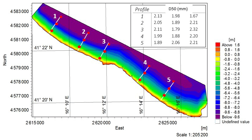
Figure 3Bathymetry of the study area (Gauss–Boaga coordinates) and cross-shore model profiles. Mean diameters (D50) measured in three locations along each profile are reported (from the coast to open sea).
The erosion or progress of the shoreline has been correlated in time with the wave energy impacting the shoreline. To this purpose, a wave hind-casting analysis for the study area has been previously run using the European Centre for Medium-Range Weather Forecasts (ECMWF) model. Statistical analysis was conducted using the ECMWF model data related to the point located in front of the coast at a distance of about 3.7 km (coordinates of the point: latitude 41.375∘, longitude 16.25∘).
Wave data have been processed from 1992 to 2013, providing that storm surges with higher intensity have N-NNE and E incoming directions, while the highest frequencies of occurrence are noted from the NNE and ESE. The derived wave with an equivalent energetic contribution used to initialize the model has a significant wave height of 0.77 m, a wave direction of 47∘ N and a wave period of 4.23 s. These data have been used as input in the LITPACK model following the Battjes and Janssen (1978) approach of wave propagation from deep water. For the present study no currents have been included in the simulation. Numerical simulations have been performed for all the three cells, referring to the years 2005, 2008, 2011, and 2013 and the model has been validated based on the available field data of coastline changes. After this, the model has predicted the shoreline evolution up to the year 2018.
Overlaying the historical shorelines of the years 1992, 1997, 2005, 2008, 2011 and 2013, the first comparative spatial analysis has been executed, to analyze and map areas of accretion and erosion in all the investigated cells. Figure 4 shows the accumulation and retreat areas in Cell I–Cell III during the overall observation period (1992–2013). A shoreline accretion is evident in Cell I and Cell III, which are in the proximity of the port of Margherita di Savoia and the port of Barletta, respectively. Conversely, in Cell II (area of Ofanto River) significant erosion has occurred.
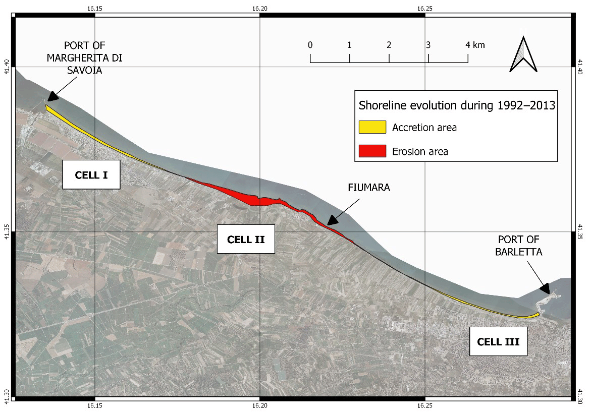
Figure 4Accumulation and retreat areas in Cell I–Cell III during the overall observation period (1992–2013).
The value of the NSM with DSAS has been returned for equally spaced transects, representing the distance between the most recent and the oldest of the two compared coastlines. A total of 577 transects, each separated by approximately 25 m, have been superimposed on the study area: 243 transects in Cell I, 44 transects in Cell II and 289 transects in Cell III. The DSAS has been applied to five time intervals for 1992–1997, 1997–2005, 2005–2008, 2008–2011 and 2011–2013. The computed shoreline rate of change has produced the following results.
4.1 Results in Cell I
Figure 5 shows that, during the years 1992–1997, in Cell I accumulation occurs in the northern area, from transect 0 to transect 110. In the central part, from transects 110 to 190, the shoreline remains quite stable. Conversely, erosion characterizes the southern area, from transects 190 to 244. During the period 1997–2005, both accumulation to the north (transects from 0 to 150) and erosion to the south (transect from 175 to 250) increase. In total, in the time interval 1992–2005, there is an accretion of about 40 m in the northern shore and an erosion of about 60 m in the southern one. The trend reverses in the successive period 2005–2008: to the north, the accretion area experiences erosion returning to values of 1997, while the erosion area experiences strong accretion to the south. During the years 2008–2011, the northern area shows stable conditions with average shoreline changes around zero (from transects 0 to 175) and the southern area shows erosion. In this period, the mean sea level had a rise of about 10 cm. Conversely, in the successive period 2011–2013 there was a decrease in the average sea level of about 2 cm (Damiani et al., 2003). This sea level variation could justify the slight accretion characterizing both the northern and southern areas in 2011–2013, as well as the analogous shoreline advancement observed in the other two investigated cells (as shown in the following). For the same temporal range, a similar tendency also characterized the beach of Senigallia, located in the central Adriatic Sea, north of the investigated site, where a general retreat was recorded (Postacchini et al., 2017).
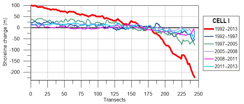
Figure 5Shoreline evolution during 1992–2013, 1992–1997, 1997–2005, 2005–2008, 2008–2011 and 2011–2013.
Consequently, in the whole investigated period 1992–2013, two different areas can be recognized in Cell I (Fig. 6): an advance area from transects 1 to 175, whose length is approximately 4300 m, and a retreat area from transects 175 to 244, whose length is about 1700 m. The overall trend in Fig. 6 clearly shows an advance of about 100 m in the northern shore and retreat of about 200 m in the southern one. Further, the modified coastline keeps its concave shape even if it undergoes a clockwise rotation. The rotation point is identified along transect 175, 4350 m from Margherita di Savoia port (Fig. 2).
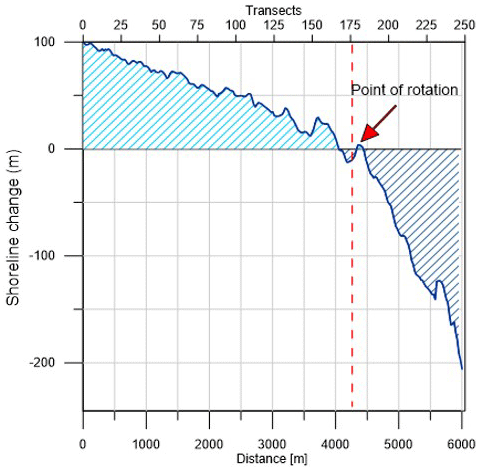
Figure 6Shoreline changes between 1992 and 2013 at Cell I. (Note that light area is accretion and dark area is erosion.)
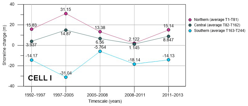
To permit a thorough comparison in the different interannual periods, Cell I is divided into three sectors (i.e., northern, central and southern), each one enclosing the same number of transects. In the following plots (Fig. 7), these sectors are indicated specifying their delimiting transects (i.e., Ti−Tj, with i and j being the number of the first and last transects of that sector). For each interannual interval, the shoreline changes computed by DSAS along each transect and inside each sector have been averaged. The corresponding averaged values are plotted in Fig. 7, with zero being the reference starting point (older available shoreline position). Measuring the shoreline rate of change with respect to this zero reference, positive values mean accretion while negative values mean erosion. Nevertheless, this data representation allows us to also estimate the relative local trend, i.e., with respect to the previous and successive temporal interval shoreline position. Thus, it is possible to evaluate both absolute and relative accretion and erosion. It is evident that the southern shoreline experiences erosion from 1992 to 2013, with a maximum shore retreat in 1997–2005. In any case, a reduced retreat, corresponding to a local advance, is noted during the years 2005–2008. The central and northern shores always display accretion, during the time interval 1992–2013. Diminished accretion is observed during 2005–2008 and 2008–2011, thus resulting in local erosion trends.
The frequent shoreline variations observed have been mostly due to human intervention, which has modified the coast, altering the beach equilibrium over the years. In Cell I, with the construction of the Margherita di Savoia port in 1992, the southern pier has retained the sediments from the Ofanto River and transported them northward by longshore currents, thus causing a remarkable advance of the shoreline.
4.2 Results in Cell II
In Cell II the shoreline evolution from 1992 to 2005 displays a progressive erosion at the Ofanto's mouth, more effective during the years 1997–2005, while a slight variation is noted to the south (Fig. 8). From 2005 to 2013 an opposite tendency occurs with accretion around the Ofanto's mouth. The trend referring to the overall period 1992–2013 highlights that the shore has suffered a severe erosion near the river mouth, with a retreat of about 250 m. It is worth noting that the erosive tendency decreases over time.
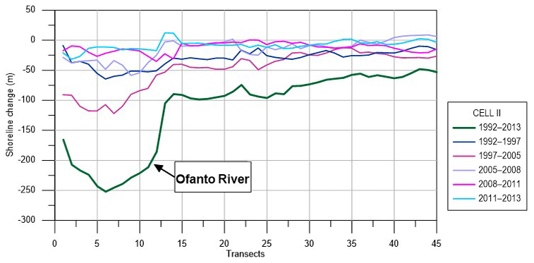
Figure 8Shoreline evolution during 1992–2013, 1992–1997, 1997–2005, 2005–2008, 2008–2011 and 2011–2013.
This is not due to reduced erosive action of waves and currents, but it is mainly due to physical changes in the Ofanto's mouth. In fact, after a deep erosive action between 1950 and 1992, because of a drastic reduction of the river solid transport, it has changed from a delta to an estuary configuration; thus it has become less erodible (Damiani et al., 2003).
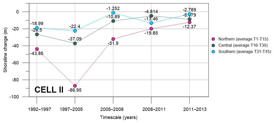
As for Cell I, Cell II has also been divided into a northern, a central and a southern sector, each one characterized by the same number of transects. The averaged shoreline changes for each sector and for the considered interannual periods are plotted in Fig. 9. A steady erosion condition is evident in all the sectors for the entire observed period, especially in the time frame 1992–2005, with the highest shoreline retreat during the years 1997–2005 in the northern sector (−86.95 m), which corresponds to the Ofanto River's mouth. In the period 2005–2011 the northern and central shores are still in a condition of retreat with respect to the zero reference, even if a process of advance establishes with reference to the previous temporal period. The analysis of the shoreline dynamics highlights that the eroded sediments in Cell II could transit through southern Cell I and finally deposit in the northern sector of Cell I.
4.3 Results in Cell III
The shoreline evolution of Cell III is displayed in Fig. 10. In the period 1992–1997, a retreat occurs in the northern part (∼10 m), while to the south the shoreline remains quite stable. A similar tendency also characterizes the period 1997–2005, with stronger erosion to the north (∼20 m).
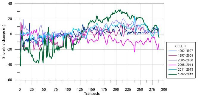
Figure 10Shoreline evolution during 1992–1997, 1997–2005, 2005–2008, 2008–2011, 2011–2013 and 1992–2013.
The successive period 2005–2011 shows an inverse tendency and accretion is noted in 2005–2008 especially. The overall trend referring to the time frame 1992–2013 illustrates a substantial erosion experienced by the northern shore with an average retreat in the shoreline position of about 30 m. Conversely, the southern shore shows a significant accumulation with an advance in the shoreline position of about 30 m. This behavior is also synthesized in Fig. 11. Namely, the shape of the northern shoreline changes from quite linear (during 1992) to concave (during 2013). Analogously to the case of Cell I, a reversal point in advance or retreat can be recognized at about 3400 m from the northern limit of Cell III. In this case, a counterclockwise rotation of the shoreline is argued (Fig. 11) and the coastline seems to evolve, preserving its concave shape. Based on the average rate of shoreline change in the northern, central and southern sectors (Fig. 12), in Cell III erosion with respect to the zero reference is noted only along with the northern sector, where a high landward excursion is evident from the year 1992 up to the year 2005. The central and southern shores are characterized by accretion, with the exception of the period 2008–2011. Similarly to Cell I, in Cell III the construction of the Barletta port has heavily modified the coastal dynamics, especially in the northern region, determining an accumulation area. Overall, in the analyzed period, the sediments of Cell II have been transported both northwestward (to Cell I) and southeastward (to Cell III), leading to accretion areas near the two ports.

Figure 11Shoreline change between 1992 and 2013 at Cell III. (Note that light area is accretion and dark area is erosion.)

Figure 12Average shoreline position in the northern, central and southern sectors of Cell III.
4.4 Assessment of beach rotation by using regression analysis and Pearson's matrix
Some useful information can be deduced by plotting in a joint graph the temporal shoreline changes that occurred within each cell (see Fig. 13a–c), with reference to the southern, central and northern sectors. The x axes report the central position of each section starting from the northern one. Particularly referring to the 1992–2013 curve, a consistent correlation emerges between southern and northern evolution for each cell. A high correlation between the southern shoreline retreat and the northern shoreline advance is evident in Cell I (Fig. 13a). In Cell II, the large erosion is proved by a linear regression model as well (Fig. 13b). Also in Cell III, a linear regression model expresses the shoreline behavior, in this case with an opposite slope in comparison to the linear regression model of Cell I, thus indicating retreat in the northern part and advance in the southern one (Fig. 13c). All these linear regression models have correlation coefficients around 0.90.
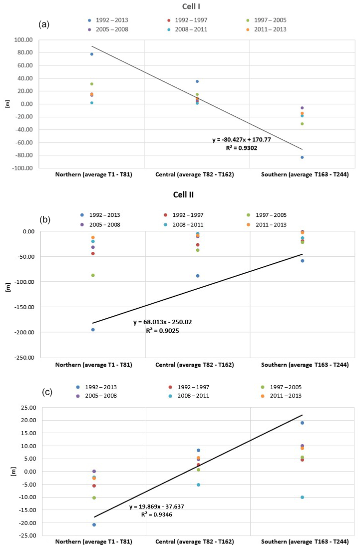
Figure 13Average variation (m) at the northern, central and southern shores in (a) Cell I, (b) Cell II and (c) Cell III for the years 1992–2013, 1992–1997, 1997–2005, 2008–2011, 2011–2013 and 2005–2008.
A further step has been made, investigating in greater detail the mutual influence of each sector on the adjacent one. Correlations between the northern–central, southern–central and southern–northern sectors are shown in Fig. 14, respectively in the left, central and right columns, for Cell I (top row), Cell II (central row) and Cell III (bottom row). In each subplot the regression equation is written, together with the corresponding R2.
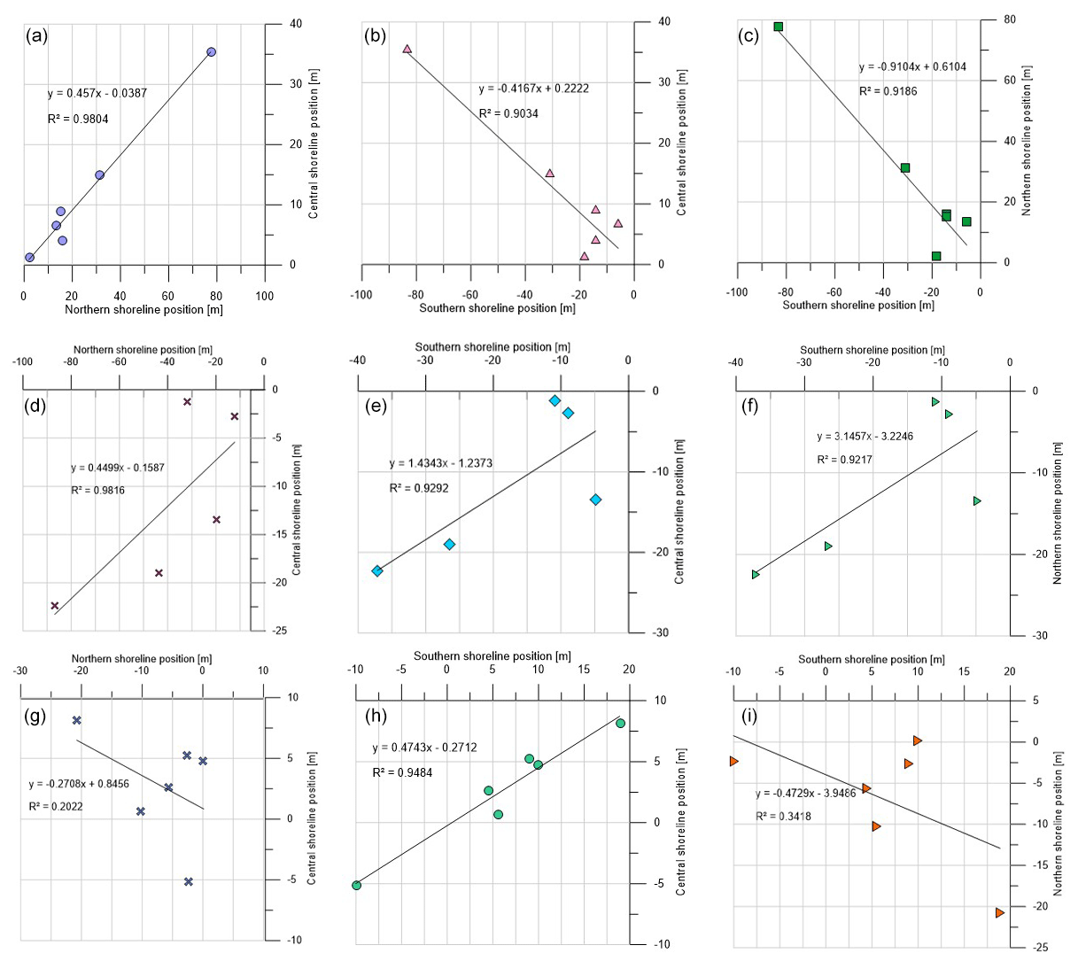
Figure 14Spatial correlations of the averaged shoreline changes during the investigated period between northern and central shorelines, southern and central shorelines, and southern and northern regions in Cell I (a–c), Cell II (d–f) and Cell III (g–i).
It is evident that in Cell I when changes occur in the northern sector, they occur with the same sign in the central sector (Fig. 14a), while when changes occur in the southern sector, they occur with the opposite sign in the central sector (Fig. 14b). However, the statistically highest negative relation observed between the southern and northern sectors is the most interesting, proving a clockwise beach rotation (Fig. 14c). In Cell II, a positive relation is estimated for all the cases: between northern and central sectors (Fig. 14d), southern and central sectors (Fig. 14e), and southern and northern sectors, confirming that in Cell II no beach rotation occurs (Fig. 14f). In Cell III a negative relation is established between the northern and central sectors (Fig. 13g), as well as between the southern and northern sectors (Fig. 14i), while a positive relation is established between the southern and central sectors (Fig. 14h). Even if in Cell III the R2 coefficients are the lowest, due to a greater data scattering, the examined trends still explain a counterclockwise beach rotation.
To thoroughly investigate these linear correlations, the Pearson correlation coefficient, r, has been computed. Specifically, it provides a measure of the linear association between two continuous variables, in this case, assumed to be some appropriate profiles, obtained in the following way. The 244 transects of Cell I have been grouped into 15 profiles (P1–P15 from north to south). Similarly, the 45 transects of Cell II have been grouped into nine profiles (P1–P9 from north to south) and the 289 transects of Cell III into 12 profiles (named P1–P12 from north to south). Each of these profiles represents the time average of the shoreline changes observed in the period 1992–2013 along a few consecutive transects. As an example, the profile P1 is the time average of the shoreline changes observed along transects T1 to T16, the profile P2 refers to transects T17 to T32 and so on. For each cell using the year 1992 as a proxy shoreline, the Pearson's correlation matrix has been calculated to attempt a best fit and compare the temporal variations along with the profiles. In addition, the Student's t test coefficient, p, has also been computed to investigate the relevance of the correlation between the profiles, which has been assumed significant for p values < 0.05. For the sake of brevity, the matrix of the Student's t test coefficient, p, has been omitted, but significant values of the correlation (characterized by p<0.05) have been written in italics in the Pearson's correlation matrixes of Tables 1–3, respectively written for Cell I–Cell III.
Table 1Pearson's correlation matrix applied to Cell I. Note: red marks positive relationships between profiles and blue marks negative relationships. Italic indicates p<0.05.
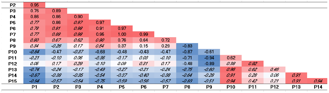
Table 2Pearson's correlation matrix applied to Cell II. Note: red marks positive relationships between profiles and blue marks negative relationships. Italic indicates p<0.05.

Table 3Pearson's correlation matrix applied to Cell III. Note: red marks positive relationships between profiles and blue marks negative relationships. Italic indicates p<0.05.

Each cell of the matrix displays the Pearson's correlation coefficient r computed between the corresponding profiles in the first vertical column and in the first bottom row. The value of r can range from −1 to 1. The sign indicates the direction of the relationship (that is, negative values imply an inverse relationship or a decreasing trend), while the absolute value indicates its strength, with larger (absolute) values meaning stronger linear relationships. The value r=0 means the absence of a linear relationship, even if other types of not linear relationships could relate the variables in any way. In Tables 1–3 positive correlations are colored in red and negative ones in blue.
In Table 1 significant positive relationships exist between the northern profiles in the range [P2–P8] so that when changes occur at one profile location they also occur on adjacent profiles. Specifically, the highest correlation is noted between P7 and P5 profiles (r=1.00). A similar scenario with positive correlations (generally moderate and high) is observed within the southern profiles [P13–P10]. The central profiles show both positive and negative correlations to be statistically irrelevant. Correlations between the remaining central profiles and both southern and northern profiles also range from negligible to moderate. The statistically high and even very high negative correlations are of uttermost interest, expressing reliable inverse relationships. The high negative correlation () between profiles P15 (extreme south) and P1 (extreme north) is stimulating as it proves the opposite trends in accretion–erosion patterns of the northern and southern limits of Cell I, thus confirming the beach rotation resulting from the regression model. A negative correlation is also observed between the south and central sectors. Where the correlation signs change within the central region (turning from profile P9 to profile P10) a fulcrum is detected; i.e., the center of the beach acts as the axis of rotation, which is consistent with observation data, corresponding to a point around 4 km to the north.
Table 2 shows mainly positive high correlations in Cell II, in northern, southern and central sectors, thus indicating that when changes take place at one profile location they also occur on the adjacent profiles. In Cell II no rotation is experienced; rather an almost uniform linear trend is noted, confirming the previous analysis.
In Cell III (Table 3), the highest positive values of r are noted for the profile couples [P3–P1] and [P4–P2] in the northernmost area and [P8–P7] and [P9–P8] in the southernmost part of Cell III, indicating a concurrent trend in the coupled profiles when advance or retraction occurs. The highest negative values of r are observed for the profile couples [P11–P1] and [P12–P1]. This means that when advance or retraction occurs in the southern region of the cell, the opposite occurs in the northern one, still indicating a beach rotation. The fulcrum in Cell III is not so evident as in Cell I, where the tendency to rotation was more noticeable.
All three simulations executed with reference to the years 2008, 2011 and 2013 have been initialized with the bathymetry of the year 2006. Simulation S1 has used the initial coastline of the year 2005 and ran until the year 2008, to compare the output coastline with 2008's observations. Simulation S2 used this validated coastline of the year 2008 as input and ran until 2011, to compare with 2011's data. Simulation S3 used the validated coastline of the year 2011 as input and has ran until 2013, to compare with 2013's observations. It is worth mentioning that, since the end of 2015, submerged barriers have been built in the study area. These structures have not been included in the modeling; hence the simulations show the evolution of the coastline disregarding the possible effects of the abovementioned works.
The comparison between GIS results and numerical results for S1–S3 simulations is shown in Fig. 15a–c for Cell I–Cell III, respectively. For each cell, the average of the observed and modeled shoreline variations in the sector (northern, central, southern) is displayed. The relative error, computed as the difference between the modeled and the measured value rated by the measured one, is also shown. These errors have been computed with reference to averaged transects, which are T1–T181 for the northern sector, T82–T162 for the central sector and T163–T244 for the southern sector. Overall, the model seems to reasonably reproduce the observed erosion–accretion rates. Specifically, a quite good agreement is noted in Cell I and Cell III, while greater errors affect Cell II, especially in the northern sector, where the Ofanto's mouth is located.
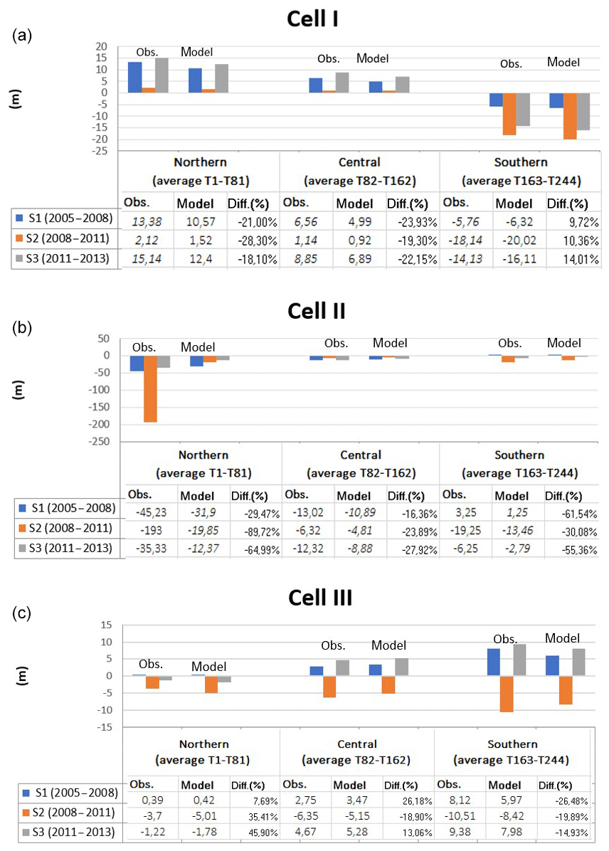
Figure 15Comparison between observation and model data for (a) Cell I, (b) Cell II and (c) Cell III. Negative values depict shoreline retreat, positive values shoreline advance (m).
In Cell I the computed error (in absolute value) is at maximum in the northern sector for the S2 run (28.3%) and minimum in the southern sector for the S1 run (9.72%). For all runs, the greatest errors are evident in the northern sector. The sign of the error highlights that the model always both underestimates the accretion of the shore occurring in the northern and central sectors of Cell I and overestimates the erosion occurring in the southern sector. In any case, a greater inaccuracy is noted in the estimation of the shoreline advance.
In Cell III the computed error (in absolute value) is at maximum in the northern sector for the S3 run (45.9 %) and minimum in the same sector for the S1 run (7.69 %). In this case, for all runs, the model overestimates both accretion and erosion in the northern sector, while it underestimates both accretion and erosion in the southern sector. Comparing this behavior of the model with that observed in the simulations of Cell I, we note that the error trend is not linear and depends on local effects.
This is even more evident when analyzing the computed error (in absolute value) in Cell II. It reaches 89.72 % in the northern sector for the S2 run, while its minimum value is 16.32 % in the central sector for the S1 run. A general underestimation of modeled values is noted in the whole Cell II in reproducing the shoreline retreat.
It is worth noting that in any case the model provides mean errors smaller than or equal to those reported in the literature for more complex models, such as multivariate linear regression models or evolutionary polynomial regression models (Goncalves et al., 2012; Bruno et al., 2019). Based on Fig. 15a and c we can state that the model suitably allows the study of the coastline evolution in the case of a slightly curved shape beach profile. In Cell II, the 2-D effects on the nearshore hydrodynamics and morphodynamics are so relevant that they cannot be accurately modeled by a one-line model, such as LITPACK.
Once the limitations of the model in the reproduction of the coastline were recognized, we used it to attempt a prediction of the shoreline evolution from 2013 to 2018. The results are displayed in Fig. 16 for Cell I–Cell III, providing the following information. In Cell I, the predicted accretion of the shoreline in the northern area is equal to 25.26 m on average and in the central area is equal to 15.43 m on average. In the southern area, erosion is predicted equal to 21.69 m on average. In Cell II, the model predicts an average erosion equal to 24.61 m in the northern area, to 16.65 m in the central area and to 10.56 m in the southern area. In Cell III, the predicted accretion of the shoreline in the southern area is 18.56 m on average, while in the central area it is 10.19 m on average. In the northern area of Cell III, an almost stable shoreline is predicted (estimated average erosion of 1.51 m).
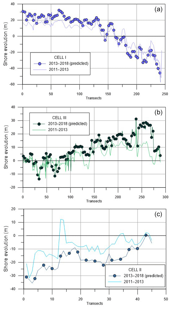
Figure 16Observed shoreline in the period 2011–2013 and predicted shoreline for the period 2013–2018 in (a) Cell I, (b) Cell II and (c) Cell III.
What is clear from this forecasting run is that the study area is evolving and the beach equilibrium has not been achieved, yet. Specifically, the clockwise beach rotation already observed in Cell I and the counterclockwise beach rotation noted in Cell III are still also expected in the simulated period 2013–2018. In Cell I and Cell III the coastline evolves while maintaining its concave shape. Further, the changes in shoreline advance and regression have the same order of magnitude of those already analyzed in previous periods.
The present study has described an approach for the assessment of beach accretion–erosion, based on the joint use of data analysis, statistical methods and one-line numerical modeling. About 18 km of the southern Adriatic coast, showing two concave beaches separated by a convex one, has been examined in the period 1992–2013.
The temporal analysis of the shoreline variation by means of GIS application has clearly shown the location of accretion and erosion areas. It has proven that in Cell I and Cell III the coastline has evolved, keeping its concave shape but rotating. A clockwise rotation has been observed in Cell I, with the formation of a northern area of sediment deposit and a southern erosion area. In Cell III a counterclockwise rotation of the coastline has produced an advance of the beach in the southern region and a retreat in the northern one. Cell II has been characterized by a progressive erosion so that the convex shape beach profile has decreased over the years. These results have also been proven by the application of the linear regression model in each cell and the computation of the Pearson's matrix, which have allowed us to thoroughly investigate correlations between northern, central and southern shoreline positions.
These data have been used to validate the numerical one-line LITPACK model, specifically in the analysis of the shoreline in the periods 2005–2008, 2008–2011 and 2011–2013. We have noted that the model is suitable in reproducing the shoreline evolution with satisfactory accuracy in the case of slightly curved shape beaches (Cell I and Cell III) while greater errors have been obtained in all runs reproducing the shoreline evolution in Cell II, due to effects not handled by the model. Even if affected by this limitation, the model has finally been used to attempt a prediction for the period 2013–2018. The result has shown that the shoreline has not reached an equilibrium yet and that the tendency already remarked in Cell I and Cell III (i.e., clockwise and counterclockwise rotation, respectively) is also confirmed in predictive terms.
The proposed procedure has shown that this joint approach in the analysis of the coastline evolution is successful, providing complete information, both qualitative and quantitative, to stakeholders and identifying areas of erosion and deposition.
Research data can be accessed by contacting Michele Mossa at his e-mail address michele.mossa@poliba.it.
EA and FDS analyzed data and wrote the paper. MM and AFP revised it and supervised the research.
The authors declare that they have no conflict of interest.
This paper was edited by Thomas Glade and reviewed by two anonymous referees.
Apulian Coastal Plan, Bollettino Ufficiale della Regione Puglia no. 31, Bollettino Ufficiale della Regione Puglia, Puglia, 29 February 2012.
Armenio, E., Meftah, M. B., Bruno, M. F., De Padova, D., De Pascalis, F., De Serio, F., Di Bernardino, A., Mossa, M., Leuzzi, G., and Monti, P: Semi enclosed basin monitoring and analysis of meteo, wave, tide and current data: Sea monitoring, in: IEEE Workshop on Environmental, Energy, and Structural Monitoring Systems (EESMS), 13–14 June 2016, Bari, Italy, 1–6, 2016.
Armenio, E., De Serio, F., and Mossa, M.: Analysis of data characterizing tide and current fluxes in coastal basins, Hydrol. Earth Syst. Sci., 21, 3441–3454, https://doi.org/10.5194/hess-21-3441-2017, 2017a.
Armenio, E., De Serio, F., Mossa, M., Nobile, B., and Petrillo, A. F.: Investigation on coastline evolution using long-term observations and numerical modelling, in: The 27th International Ocean and Polar Engineering Conference, International Society of Offshore and Polar Engineers, 25–30 June 2017, San Francisco, California, USA, 2017b.
Armenio, E., De Padova, D., De Serio, F., and Mossa, M.: Monitoring system for the sea: Analysis of meteo, wave and current data, in: IMEKO TC19 Workshop on Metrology for the Sea, MetroSea, 25–30 June 2017, San Francisco, California, USA, 2017c.
Armenio, E., De Serio, F., and Mossa, M.: Environmental technologies to safeguard coastal heritage, SCIRES-IT-SCIentific RESearch and Information Technology, 8, 61–78, 2018.
Battjes, J. A. and Janssen, J. P. F. M.: Energy loss and set-up due to breaking of random waves, Coast. Eng., 1, 569–587, 1978.
Blossier, B., Bryan, K. R., and Winter, C.: Simple Pocket Beach Rotation Model Derived from Linear Analysis, in: Proc. Coastal Sediments 2015, San Diego, USA, 2015.
Boak, E. H. and Turner, I. L.: The Shoreline detection-definition problem: a review, J. Coast. Res., 21, 688–703, 2005.
Bonaldo, D., Antonioli, F., Archetti, R., Bezzi, A., Correggiari, A., Davolio, S., De Falco, G., Fantini, M., Fontolan, G., Furlani, S., Gaeta, M. G., Leoni, G., Lo Presti, V., Mastronuzzi, G., Pillon, S., Ricchi, A., Stocchi, P., Samaras, A. G., Scicchitano, G., and Carniel, S.: Integrating multidisciplinary instruments for assessing coastal vulnerability to erosion and sea level rise: lessons and challenges from the Adriatic Sea, Italy, J. Coast. Conserv., 23, 19–37, 2019.
Brooks, S. M. and Spencer, T.: Temporal and spatial variations in recession rates and sediment release from soft rock cliffs, Suffolk coast, UK, Geomorphology, 124, 26–41, 2010.
Bruno, M. F., Molfetta, M. G., Pratola, L., Mossa, M., Nutricato, R., Morea, A. B., Nitti, D. O., and Chiaradia, M. T.: A combined approach of field data and earth observation for coastal risk assessment, Sensors, 19, 1399, https://doi.org/10.3390/s19061399, 2019.
Bryan, K. R. Foster, R., and MacDonald, I.: Beach Rotation at Two Adjacent Headland-Enclosed Beaches, J. Coast. Res., 2, 2095–2100, 2013.
Chiaradia, M. T., Francioso, R., Matarrese, R., Petrillo, A. F., Ranieri, G., and Urrutia, C.: Estrazione semi-automatica della linea di costa da immagini satellitari ad alta risoluzione: valutazione ed applicabilità, Collana Editoriale di Studi e Ricerche dell'Autorità di Bacino della Basilicata, Italy, 9 pp., 2008.
Cutter, S. L., Barnes, L., Berry, M., Burton, C., Evans, E., Tate, E., and Webb, J.: A place-based model for understanding community resilience to natural disasters, Global Environ. Change, 18, 598–606, 2008.
Damiani, L., Petrillo, A. F., and Ranieri, G.: The erosion along the apulian coast near the Ofanto river, in: Coastal Engineering VI, edited by: Brebbia, C. A., Almorza, D., and Lopez-Aguayo, F., available at: https://www.witpress.com/elibrary/wit-transactions-on-the-built-environment/70 (last access: 1 September 2019), 2003.
Davidson, N. C., Laffoley, D. D., Way, L. S., Key, R., Drake, C. M., Pienkowski, M. W., Mitchell, R., and Duff, K. L.: Nature conservation and estuaries in Great Britain, Nature Conservancy Council, Peterborough, UK, 1991.
Dean, R. G. and Dalrymple, R. A.: Coastal Processes with Engineering Applications, Cambridge University Press, Cambridge, 2004.
Deigaard, R., Fredsoe, J., and Hedegaard, I. B.: Suspended sediment in the surf zone, J. Waterway Port Coast. Ocean Eng., 112, 115–128, 1986a.
Deigaard, R., Fredsoe, J., and Hedegaard, I. B.: Mathematical model for littoral drift, J. Waterway Port Coast. Ocean Eng., 112, 351–369, 1986b.
De Padova, D., De Serio, F., Mossa, M., and Armenio, E.: Investigation of the current circulation offshore Taranto by using field measurements and numerical model, in: Proc. 2017 IEEE International Instrumentation and Measurement Technology Conference, Torino, Italy, 2017.
De Serio, F. and Mossa, M.: Streamwise velocity profiles in coastal currents, J. Environ. Fluid. Mech., 14, 895–918, 2014.
De Serio, F. and Mossa, M.: Assessment of hydrodynamics, biochemical parameters and eddy diffusivity in a semi-enclosed Ionian basin, Deep-Sea Res. Pt. II, 133, 176–185, 2016.
De Serio, F., Armenio, E., Mossa, M., and Petrillo, A.: How to Define Priorities in Coastal Vulnerability Assessment, Geosciences, 8, 415, 2018.
DHI – Danish Hydraulic Institute: Software manual, Horlsholm, Denmark, 2016.
Dolan, R., Hayden, B. P., and Felder, W.: Systematic variations in inshore bathymetry, J. Geol., 85, 129–141, 1977.
Dolan, R., Fenster, M. S., and Holme, S. J.: Temporal analysis of shoreline recession and accretion, J. Coast. Res., 7, 723–744, 1991.
Douglas, B. C. and Crowell, M.: Long-term shoreline position prediction and error propagation, J. Coast. Res., 16, 145–152, 2000.
Elfrink, B., Christensen, ED., Brøker, I., Gonella, M., and Morelli, M.: Local Morphological Evolution of the Coast in the Upper Adriatic Sea. Design and Management Strategies to Control Coastal Erosion, in: CENAS, edited by: Gambolati, G., Springer, the Netherlands, 263–289, 1998.
Foster, E. R. and Savage, R. J.: Methods of Historical Shoreline Analysis, in: Proc. Coastal Zone '89, ASCE, New York, USA, 1989.
Fredsoe, J., Andersen, O. H., and Silberg, S.: Distribution of suspended sediment in large waves, J. Waterway Port Coast. Ocean Eng., 111, 1041–1059, 1985.
Frey, A. E., Connell, K. J., Hanson, H., Larson, M., Thomas, R. C., Munger, S., and Zundel, A.: GenCade Version 1 Model Theory and User's Guide, Report No. ERDC/CHL-TR-12-25, US Army Corps of Engineers, Vicksburg, MS, USA, 2012.
Genz, F., Lessa, G. C., and Cirano, M.: The impact of an extreme flood upon the mixing zone of the Todos Santos Bay, Northeastern Brazil, J. Coast. Res., 39, 707–712, 2006.
Goncalves, R. M., Awange, J. L., Krueger, C. P., Heck, B., and dos Santos, C. L.: A comparison between three short-term shoreline prediction models, Ocean Coast. Manage., 69, 102–110, 2012.
González-Villanueva, R., Costas, S., Pérez- Arlucea, M., Jerez, S., and Trigo, R. M.: Impact of atmospheric circulation patterns on coastal dune dynamics, NW Spain, Geomorphology, 185, 96–109, 2013.
Jabaloy-Sánchez, A., Lobo, F. J., Azor, A., Martín- Rosales, W., Pérez-Peña, J. V., Bárcenas, P., Macías, J. M., Fernández-Salas, L. M., and Vázquez- Vílchez, M.: Six thousand years of coastline evolution in the Guadalfeo deltaic system (southern Iberian Peninsula), Geomorphology, 206, 374–391, 2014.
Katz, O. and Mushkin, A.: Characteristics of sea-cliff erosion induced by a strong winter storm in the eastern Mediterranean, Quaternary Res., 80, 20–32, 2013.
Oyedotun, T. D. T.: Shoreline Geometry: DSAS as a Tool for Historical Trend Analysis, in: Geomorphological Techniques, chap. 3, Sect. 2.2 (2014), ISSN 2047-0371, available at: https://www.geomorphology.org.uk/sites/default/files/geom_tech_chapters/3.2.2_ShorelineGeometry.pdf (last access: 1 September 2019), 2014.
Postacchini, M., Soldini, L., Lorenzoni, C., and Mancinelli, A.: Medium-term dynamics of a middle Adriatic barred beach, Ocean Sci., 13, 719–734, https://doi.org/10.5194/os-13-719-2017, 2017.
Samaras, A. G., Gaeta, M. G., Miquel, A. M., and Archetti, R.: High-resolution wave and hydrodynamics modelling in coastal areas: operational applications for coastal planning, decision support and assessment, Nat. Hazards Earth Syst. Sci., 16, 1499–1518, https://doi.org/10.5194/nhess-16-1499-2016, 2016.
Schoonees, J. S. and Theron, A. K.: Evaluation of 10 cross-shore sediment transport/morphological models, Coast. Eng., 25, 1–41, 1995.
Short, A. D. and Trembanis, A. C.: Decadal scale patterns in beach oscillation and rotation Narrabeen beach, Australia-Time series, PCA and Wavelet analysis, J. Coast. Res., 20, 523–532, 2004.
Termini, D.: River processes and links between fluvial and coastal systems in a changing climate, available at: https://cmgds.marine.usgs.gov/publications/DSAS/of2008-1278/ (last access: 1 September 2019), 2018.
Thébaudeau, B., Trenhaile, A. S., and Edwards, R. J.: Modelling the development of rocky shoreline profiles along the northern coast of Ireland, Geomorphology, 203, 66–78, 2013.
Thieler, E. R. and Danforth, W. W.: Historical shoreline mapping (I) Improving techniques and reducing positioning errors, J. Coast. Res., 10, 549–563, 1994a.
Thieler, E. R. and Danforth, W. W.: Historical shoreline mapping (II) Application of the Digital Shoreline Mapping and Analysis Systems (DSMS/DSAS) to shoreline change mapping in Puerto Rico, J. Coast. Res., 10, 600–620, 1994b.
Thieler, E. R., Himmelstoss, E. A., Zichichi, J. L., and Ergul, A.: The Digital Shoreline Analysis System (DSAS) version 4.0 – an ArcGIS extension for calculating shoreline change, Report No. 2008-1278, US Geological Survey, Reston, 2009.
Thomas, R. C. and Frey, A. E.: Shoreline change modeling using one-line models: General model comparison and literature review, Report No. ERDC/CHL CHETNII-55, US Army Corps of Engineers, Vicksburg, MS, USA, 2013.
Torresan, S., Critto, A., Rizzi, J., and Marcomini, A.: Assessment of coastal vulnerability to climate change hazards at the regional scale: the case study of the North Adriatic Sea, Nat. Hazards Earth Syst. Sci., 12, 2347–2368, https://doi.org/10.5194/nhess-12-2347-2012, 2012.
Young, A. P., Flick, R. E., O'Reilly, W. C., Chadwicj, D. B., Crampton, W. C., and Helly, J. J.: Estimating cliff retreat in southern California considering sea level rise using a sand balance approach, Mar. Geol., 348, 15–26, 2014.