The use of historical information for regional frequency analysis of extreme skew surge

The design of effective coastal protections requires an adequate estimation of the annual occurrence probability of rare events associated with a return period up to 10³ years. Regional frequency analysis (RFA) has been proven to be an applicable way to estimate extreme events by sorting regional data into large and spatially distributed datasets. Nowadays, historical data are available to provide new insight on past event estimation. The utilisation of historical information would increase the precision and the reliability of regional extreme's quantile estimation. However, historical data are from significant extreme events that are not recorded by tide gauge. They usually look like isolated data and they are different from continuous data from systematic measurements of tide gauges. This makes the definition of the duration of our observations period complicated. However, the duration of the observation period is crucial for the frequency estimation of extreme occurrences. For this reason, we introduced here the concept of “credible duration”. The proposed RFA method (hereinafter referenced as FAB, from the name of the authors) allows the use of historical data together with systematic data, which is a result of the use of the credible duration concept.

1 Introduction

Flood risk is a noteworthy threat for anthropic and industrial settlement along the coast. Coastal defence constructions have to withstand extreme events. Therefore, in this context, a statistical estimation of extreme marine variables (such as sea levels or skew surges, the difference between the maximum observed sea level and the maximum predicted astronomical tide level during a tidal cycle; Simon, 2007; Weiss, 2014) occurrence probability is necessary. These variables associated with high return periods (up to 1000 years; ASN, 2013) are estimated by statistical methods linked to the extreme value theory (EVT) (Fréchet, 1928; Gnedenko, 1943; Gumbel, 1958; Picklands, 1975; Coles, 2001).

In the past, time series recorded at a single site had been used to estimate return levels for marine hazards. However, these extreme quantiles are linked to huge estimation uncertainties due to local recordings being too short (typically 30 to 50 years long). A greater amount of data is therefore necessary to obtain reliable estimations of extreme marine hazards.

For this reason and thanks to the availability of several local datasets, the regional frequency analysis (RFA) is employed to reduce statistical uncertainties, allowing the use of bigger extreme samples. The primary purpose of RFA is to cluster different locations in a region and to use all the data together (Cunnane, 1988; Hosking and Wallis, 1997; Van Gelder and Neykov, 1998; Bernardara et al., 2011; Weiss, 2014). RFA is based on the index flood principle (Dalrymple, 1960) that introduces a local index for each site in order to preserve their peculiarities in a region. A regional distribution can be defined only after checking its statistical homogeneity (Hosking and Wallis, 1997). The probability distribution of extreme values must be the same everywhere in the region to allow the fitting of a probability distribution with a big data sample. Several applications exist for marine variables, although these are mostly for skew surges (Bernardara et al., 2011; Bardet et al., 2011; Weiss et al., 2013).

Specifically, Weiss (2014) proposed a RFA approach to treat extreme waves and skew surges. According to this approach, homogeneous regions are first built relying on typical storm footprints and their statistical homogeneity is subsequently tested. The addition of physical elements allows for the inclusion of to regions that are both physically and statistically homogeneous. Furthermore, this methodology, and the pooling method in particular, yields an equivalent regional duration in years that enables the evaluation of the return periods of extreme events.

As proved in hydrology, extending datasets with historical data or paleofloods is an alternative way to reduce uncertainties in the estimation of extremes (Benson, 1950; Condie and Lee, 1982; Cohn, 1984; Stedinger and Cohn, 1986; Hosking and Wallis, 1986a, 1986b; Cohn and Stedinger, 1987; Stedinger and Baker, 1987; Ouarda et al., 1998; Benito et al., 2004; Reis and Stedinger, 2005; Payrastre et al., 2011; Sabourin and Renard, 2015) as well as representing better potential outliers. Previous works on local sea levels (Val Gelder, 1996; Bulteau et al., 2015) and on local skew surges (Hamdi et al., 2015) pointed out that the incorporation of historical data leads to a positive effect on extreme frequency analysis.

The combination of these two approaches increases the amount of available data allowing to get better extreme return levels. The use of extraordinary floods events in RFA has already been explored by Nguyen et al. (2014) for peak discharges and Hamdi et al. (2016) have explored it in the frame of oceanic and meteorological variables.

In this study, we investigate the use of historical data in RFA of systematic measurements of skew surge levels. The proposed FAB method (a declination of RFA using credible duration) allows the estimation of reliable extreme skew surge events by taking into account all the available non-systematic records of skew surge levels. Specifically, historical data are defined as all of the skew surge events that were not recorded by a tide gauge, and consequently, systematic data are all the measurements of skew surge recorded by tide gauge. One obvious and very promising way of collecting information not recorded by a tide gauge is to investigate and reconstruct historical events that occurred before the starting date of gauge observations. This activity is also known as data archaeology and has been demonstrated very promising and useful for several study in the literature. However, this definition also includes isolated data points reconstructed during gaps in the systematic measurements. This is because statistically speaking they could be treated similarly to the isolated data reconstructed from before the gauged period. To find historical events it is thus necessary to go back in time and look for information before the gauging period or during each data gap in a time series. During extreme storms, tide gauge may be affected by a partial or total failure in the sea level measurements and so this kind of event cannot always be detected. Thanks to non-systematic records, we can hold a numerical value to these ungauged extreme events. This allows to use a larger number of storms in the statistical assessment of the extreme skew surges.

Baart et al. (2011) pointed out the hitch in recovering accurate historical information. A historical event is the result of a wide investigation of several qualitative and quantitative sources. Historical data are collected from different sources as newspapers of the period, archives, water marks, palaeographic studies etc. For this reason, each historical data has its own origin and its quality has to be checked (Barriendos et al., 2003). Therefore, a critical analysis of historical data must be performed before applying a statistical approach.

Using historical data with time series data recorded by a tide gauge is not a simple process. Extreme statistical analysis requires a knowledge of the time period for which all the events above an extreme threshold are known (Leese, 1973; Payrastre et al., 2011). For the gauged, or preferably, systematic data, this time is represented by the recording period (i.e. systematic duration). As historical data are isolated data points, the duration of the observation is not defined. What happened during the time period between two or more past extreme events remains unknown. However, the coverage period estimation of historical data is a key step in extreme value statistical models (Prosdocimi, 2018). Reasonable computation of historical duration is the base of reliable statistical estimation of rare events.

In the past, to overcome these issues the perception threshold concept has been introduced. The perception threshold represents the minimum value over which all the historical data are reported and documented (Payrastre et al., 2011; Payrastre et al., 2013). The hypothesis is thus set that all the events over the perception threshold must have been recorded and the time period without records corresponds to time period without extreme events. This allows the estimation of the coverage period and the indirect assumption that the collected historical data are exhaustive throughout the coverage period assessed. So far, the perception threshold has allowed the use of historical information in extreme frequency analysis (Payrastre et al., 2011; Payrastre et al., 2013; Bulteau et al., 2015) but the hypothesis for using this approach seems sometimes difficult to prove.

Indeed, the perception threshold is usually defined equal to a historical event value, based on the principles that, if any other historical event would have occurred it would have been recorded (Payrastre et al., 2011; Bulteau et al., 2015). This is quite a sweeping hypothesis, which is difficult to verify and validate. Moreover, the duration associated to the perception threshold is usually defined as the duration between the oldest historical data and the start of the systematic series (Payrastre et al., 2011; Hamdi et al., 2015).

The main point of difference in this paper is the proposal of a new approach in order to deal with these questions in a more satisfactory way.

Note that the new approach is required for the application of the RFA, at least in the POT approaches (Van Gelder and Neykov, 1998; Bernardara et al., 2011; Bardet et al., 2011; Weiss et al., 2014b). Indeed, the definition of the perception threshold as equal to a historical value precludes the possibility of using the RFA methodology proposed by Weiss (2014). Specifically, in Weiss regional methodology, the number of extreme events per year λ must be equal in each site of a region in order to estimate a regional distribution. This is impossible to achieve if the threshold is linked to the characteristics of the local observations.

In addition, when historical information (i.e. non-systematic data) is collected during a total failure of tide gauge, this influences the frequency of the event. One could only re-estimate λ if the credible duration is re-estimated (for details, see the Sect. 2).

In order to deal with these questions in this paper, a different approach is proposed to estimate the equivalent duration of historical data. This evaluation is based on the hypothesis that the frequency of the extreme events is not changing significantly in time. In other words, the average number of extreme events should be the same (obviously this has to be carefully verified and demonstrated case by case). In this way, we can assess the coverage period of historical data. Based on the frequency value of systematic storms occurrence, our hypothesis introduces a physical and tangible element in the estimation of historical duration. For this reason, we state that this advantage allows us to supplant the concept of a perception threshold providing by a credible estimation of the unknown historical duration used to estimate the extreme quantiles.

Thanks to this new concept of duration in this study, the FAB methodology is developed in order to use historical data and systematic data together in a RFA of extreme events. This methodology, described in detail in Sect. 2, is applied to the extreme skew surges given by 71 tide gauges located on the British, French and Spanish coasts and 14 historical collected skew surges is shown in Sect. 4. In addition, a functional example on the computation of credible duration is illustrated in Sect. 3.

2 FAB Methodology

2.1 The concept of credible duration

In the extreme value analysis (EVA) of natural hazards, the estimations of extreme quantiles are performed by applying statistical tools to a dataset of extreme variables. Usually, these datasets of extremes can be generated from continuous time series data or by taking extremes as the maximum value in several predefined time blocks (block maxima approach) or fixing a sampling threshold (peak-over-threshold (POT) approach).

Based on a POT approach, our study examines datasets of skew surges. From now on, we use skew surge as our chosen extreme variable but all concepts that we will describe can be extended also to other natural hazards.

In the POT framework, an extreme sampling threshold has to be considered in order to extract the dataset of extreme skew surges from continuous time series data of systematic skew surges recorded by tide gauge. In this way, the extreme sample is created and the extreme quantiles computation of skew surge can be performed according to the statistical distribution used. The relationship between return periods T and quantiles x_T is expressed as follows:

$$\begin{array}{}\text{(1)}& P\left(X>x_T\right)={\displaystyle \frac{\mathrm{1}}{\mathit{\lambda }T}},\end{array}$$

where P(X>x_T) is the exceedance probability of x_T or the probability that in every λT years an event X, stronger than x_T, will occur. By using Eq. (1), the results can be illustrated through a return level plot.

The variable λ represents the number of skew surge events per year that exceed the sampling threshold. In other words, λ is the frequency of storm occurrence and it can be expressed as the ratio of the number of skew surges n over the sampling threshold to the recording time of systematic skew surge measurements in years d (hereafter called systematic duration).

$$\begin{array}{}\text{(2)}& \mathit{\lambda }={\displaystyle \frac{n}{d}}\end{array}$$

Knowledge of n and d is necessary to compute the frequency of extreme skew surges occurrence λ and to estimate extreme quantiles of skew surges. In other words, a duration estimation is needed to transform the probability [no units] in frequency [time⁻¹ dimension].

When historical skew surges are available, the computation of λ is a complex topic. In fact, although the number of historical data n_hist over the sampling threshold is known, we do not have any information on what happens during non-gauged periods. It is thus impossible to define a duration over which the n_hist data are observed. In other words, regardless of the selection of sampling threshold value, we need this information to define the frequency of occurrence of events over the threshold (see the Eq. 2). We called the missing information “historical duration” d_hist, or in other words, the time period for which historical skew surges above the sampling threshold are estimated to be exhaustively recorded to the best of our knowledge. The inclusion of historical data in a systematic dataset of extreme skew surge is shown as an example in Fig. 1. It needs the formulation of a credible hypothesis in order to estimate the duration of the whole dataset composed by systematic and historical records.

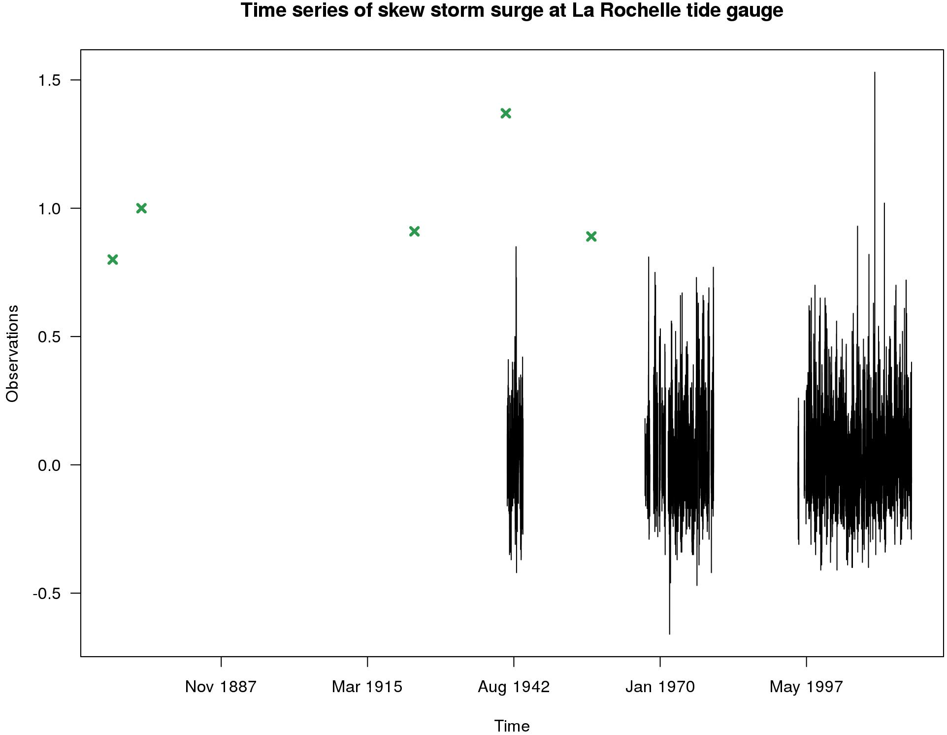
Figure 1 Illustrative example of the skew surge dataset at the La Rochelle tide gauge. In black the systematic skew surge and in green the historical isolated data points (non-systematic data) are shown.

Taking advantage of the perfect knowledge of systematic skew surges, the basic hypothesis proposed here for the computation of historical duration is that the frequency of storms λ remains unchanged over time. More precisely, λ_syst, namely the number of systematic skew surges per year over the sampling threshold, is supposed to be equal to λ_hist, namely the number of historical skew surges per year over the same sampling threshold.

$$\begin{array}{}\text{(3)}& \mathit{\lambda }={\mathit{\lambda }}_{\mathrm{syst}}={\mathit{\lambda }}_{\mathrm{hist}}\end{array}$$

Equation (3) is in accordance with the lack of a significant trend on the extreme skew surges frequency during the second part of the 19th, 20th and the first part of 21st century in the regions considered in this study (Fig. 5).

According to current scientific literature, based on past observations, frequency of storms has no defined trend (Hanna et al., 2008; Barring and Fortuniak, 2009; MICORE Project, 2009). Therefore, the hypothesis that storm frequency is constant has been assumed. No significant trends are detected in terms of magnitude or frequency of storms between 1780 and 2005 in the North Atlantic and European regions since the Dalton minimum (Barring and Fortuniak, 2009). Over the past 100 years in the North Atlantic basin, no robust trends in annual numbers of tropical storms, hurricanes and major hurricanes have been identified by the last IPCC report of 2013. Hanna et al. (2008), Matulla et al. (2008) and Allan et al. (2009) state that observations have no clear trends over the past century or longer with substantial decadal and longer fluctuations with the exceptions of some regional and seasonal trends (Wang et al., 2009, 2011). Moreover, MICORE (2009) in the “Review of climate change impacts on storm occurrence” affirms that results from coastal areas do not detect any significant trend in the frequency of storms for the existing and available datasets.

Therefore, the hypothesis that storm frequency is constant may be a reasonable working hypothesis for demonstrating this approach. Obviously, it is crucial to test this hypothesis before the application of the approach in the present state to any new dataset. Note that the methodology could be adapted quickly in the future for non-stationary datasets, where the introduced concept can be adjusted. For skew surges, the validity this hypothesis is ensured.

The assumption that the annual frequency of skew surges has been constant in Europe during the last two centuries is warranted by the several references mentioned above. A solid check must be done for other marine variables to know if they can fit this hypothesis as well.

A new duration of observation d_cr is defined as “credible” (i.e. based on credible hypothesis) considering a steady λ. This novelty is expressed as follows:

$$\begin{array}{}\text{(4)}& d_{\mathrm{cr}}={\displaystyle \frac{n_{\mathrm{tot}}}{\mathit{\lambda }}}={\displaystyle \frac{n_{\mathrm{syst}}+n_{\mathrm{hist}}}{\mathit{\lambda }}}={\displaystyle \frac{n_{\mathrm{syst}}}{\mathit{\lambda }}}+{\displaystyle \frac{n_{\mathrm{hist}}}{\mathit{\lambda }}}.\end{array}$$

Equation (4) shows how the number of extreme data is divided in two sides according to the nature of data: n_syst is the number of extreme systematic data above the sampling threshold u and n_syst is the number of extreme historical data over the same threshold u. Therefore, the credible duration also depends on the sampling threshold value.

Moreover, this splitting indirectly provides the coverage period of historical skew surges in addition to the duration of recorded data. The historical side of the duration $d_{{\mathrm{cr}}^{\mathrm{hist}}}$ can be formulated as follows:

$$\begin{array}{}\text{(5)}& d_{\mathrm{cr}}^{\mathrm{hist}}={\displaystyle \frac{n_{\mathrm{hist}}}{\mathit{\lambda }}}.\end{array}$$

The coverage period on average that every historical skew surge holds is called associated duration d_cr,ass.

$$\begin{array}{}\text{(6)}& d_{\mathrm{cr},\mathrm{ass}}={\displaystyle \frac{d_{\mathrm{cr}}^{\mathrm{hist}}}{n_{\mathrm{hist}}}}={\displaystyle \frac{\mathrm{1}}{\mathit{\lambda }}}\end{array}$$

Equation (6) displays how the associated duration can be evaluated just by knowing λ. Therefore, every extreme data not originated from a recorded time series has an associated duration. This is also the case for historical events that occurred during a time gap in gauged skew surges series.

A functional example is illustrated in Sect. 3 in order to explain all of the notions put forth up to this point and their relevance to the sampling threshold choice.

2.2 The use of credible duration in RFA framework

Weiss (2014) defined a methodology to fit a regional probability distribution for sea extreme variables. This approach enables the putting together of data from different locations and the forming of regions. The probability distribution of extreme skew surges must be the same inside a region. Thus, the extreme data of the same region are gathered together through the use of a normalisation parameter, which preserves the peculiarities of each site and the regional probability distribution defined as such. The formation of regions based on typical storm footprints (Weiss et al., 2013) is used to create physically and statistically homogeneous regions and it leads to knowledge of a master component of this regional process: the regional effective duration D_eff.

The regional effective duration D_eff represents the effective duration (in years), filtered of any intersite dependence, in which the number of regional data N_r are observed. D_eff is defined as the product of the degree of regional dependence φ[1;N] and the mean of local durations:

$$\begin{array}{}\text{(7)}& D_{\mathrm{eff}}=\mathit{\phi }\times \stackrel{\mathrm{‾}}{d}={\displaystyle \frac{{\mathit{\lambda }}_{\mathrm{r}}}{\mathit{\lambda }}}\stackrel{\mathrm{‾}}{d}={\displaystyle \frac{N_{\mathrm{r}}}{\mathit{\lambda }}},\end{array}$$

where λ_r is the number of regional storms per year ${\mathit{\lambda }}_{\mathrm{r}}=N_{\mathrm{r}}/\stackrel{\mathrm{‾}}{d}$ and $\stackrel{\mathrm{‾}}{d}$ is the mean of local observations' duration of the N regional sites: $\stackrel{\mathrm{‾}}{d}=\sum _{i=\mathrm{1}}^N{d}_i/N$.

The local frequency of storms λ must be the same across the region. More details about the D_eff are clarified in Weiss et al. (2014b) for the classic RFA approach, which is set for systematic data.

The knowledge of the regional sample duration, as exposed by a generic frequency analysis in the previous paragraph of this section, is a required factor. In fact, the evaluation of the regional return period T_r of a particular regional quantile $x_{T_{\mathrm{r}}}$ is expressed as in Eq. (8) as follows:

$$\begin{array}{}\text{(8)}& T_{\mathrm{r}}={\displaystyle \frac{\mathrm{1}}{{\mathit{\lambda }}_{\mathrm{r}}P\left(X_s>x_{T_{\mathrm{r}}}\right)}},\end{array}$$

where $P\left(X_s>x_{T_{\mathrm{r}}}\right)$ is the probability that a storm s impacts at least one site in the region with a normalised intensity greater than $x_{T_{\mathrm{r}}}$. Therefore, thanks to the regional distribution F_r, the local return period of the storm s is calculated as follows:

$$\begin{array}{}\text{(9)}& T={\displaystyle \frac{\mathrm{1}}{\mathit{\lambda }\left(\mathrm{1}-F_{\mathrm{r}}\left(x_{T_{\mathrm{r}}}\right)\right)}}.\end{array}$$

In addition, Weiss et al. (2014b) use for the computation of the empirical local return periods a Weibull plotting position. This element is correlated with the regional duration D_r:

$$\begin{array}{}\text{(10)}& {\stackrel{\mathrm{̃}}{T}}_{s,\mathrm{loc}}={\displaystyle \frac{D_{\mathrm{r}}+\mathrm{1}}{n_{\mathrm{r}}+\mathrm{1}-\text{rank}\left(s\right)}},\end{array}$$

here the biggest storm s_max of the regional sample is linked to a local return period thanks to D_r.

However, the need to employ historical data in the extreme analysis has been considered as highly relevant by scientific community to get reliable quantiles and to not miss significant information. In the RFA, the use of historical records is allowed by the new notion of credible duration. A new way to process historical skew surges at regional scale is introduced. The addition of one or more historical skew surges in one or more sites of a region requires the knowledge of the duration of each site. Thanks to the credible duration concept applied previously to a single site, a coverage period for both types of data can be evaluated. It allows switching from the notion of the regional effective duration D_r,eff to the regional credible duration D_r,cr:

$$\begin{array}{}\text{(11)}& D_{\mathrm{r},\mathrm{cr}}=\mathit{\phi }\times \stackrel{\mathrm{‾}}{d}=\mathit{\phi }\sum _{i=\mathrm{1}}^N{\displaystyle \frac{d_{i,\mathrm{cr}}}{N}}.\end{array}$$

Regional credible duration depends also on the degree of regional dependence φ that increases when the data are independent. Moreover, Eq. (11) shows that a local duration surplus consequently brings an excess of the coverage period of regional sample. With some simplifications, the Eq. (11) can thus be reformulated as follows:

$$\begin{array}{}\text{(12)}& D_{\mathrm{r},\mathrm{cr}}={\displaystyle \frac{{\mathit{\lambda }}_r}{\mathit{\lambda }}}\stackrel{\mathrm{‾}}{d}={\displaystyle \frac{N_r}{\mathit{\lambda }}}.\end{array}$$

The lack of a trend on storms' frequency is a necessary condition to assume a steady λ. If this hypothesis is satisfied, the regional credible duration can be computed.

The regional frequency analysis of skew surges including historical data, or FAB method, can be performed and these two combined approaches ensure better estimations of extreme values.

3 Illustration of credible duration

In order to better illustrate the concept of credible duration and how it varies according to different thresholds, a specific illustration on connection between these variables is described in this section by the example shown in Fig. 1.

Figure 1 shows the functional example of the whole skew surge series recorded at the La Rochelle tide gauge (France). Systematic skew surges are represented by the continuous series of data plotted in black from about 1940 to 2017. They are observed during a fixed period equal to the recording time period, in this case, 32.88 years.

The historical skew surges are artificial data generated by ourselves for this descriptive illustration and they are represented as green cross points. As they are not supposed to be obtained by continuous systematic records of skew surge measurements, the duration of their support is unknown.

As expressed above, d_cr and in particular $d_{\mathrm{cr}}^{\mathrm{hist}}$ depends on the sampling threshold value u. Equations (4) and (5) show this dependence through the λ value.

The application of the new proposed concept allows the computation of the historical duration of skew surges that represents a basic way to take into account the historical data on the estimation of extreme values.

Although the period of systematic observation is known and fixed by tide gauge's records, the coverage period of historical observations is associated with the value of sampling threshold u. The λ value is computed from the systematic measurements (Eq. 2). As a result of the hypothesis that the frequency of storms λ has no trend (Eq. 3), this λ value is then used to compute the duration of the historical records. Moreover, the hypothesis of Eq. (3) leads to different values of historical duration for each λ selected value and consequently, for each likely sampling threshold. Four cases of different values of high sampling threshold are examined (Fig. 2 and Table 1); these particular cases are chosen in order to let us know the effects of different sampling thresholds on the computation of the credible duration.

Figure 2 Skew surge dataset of Sect. 3 (composed of systematic and historical data) used in the computation of credible duration with 4 different thresholds u_c1, u_c2, u_c3, u_c4. The four sampling thresholds u_c are used linked to a rising value o λ (λ_c1= 0.5, λ_c2= 0.23, λ_c3= 0.2, λ_c4= 0.07).

Table 1 Summary table of several variables involved in the computation of credible duration for 4 different cases of study.

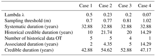
Case 1 uses a sampling threshold u_c1 corresponding to 0.5 extremes per year (λ= 0.5) and lead to a credible duration of 42.88 years (Table 1). A higher threshold u_c2 is used in Fig. 2 for the Case 2 (λ= 0.23) and the credible duration grows until 54.62 years as the number of historical data over the threshold does not change. In Case 3, the threshold (u_c3) increases (λ= 0.2) but the credible duration decreases (52.88 years) because the smallest value of historical skew surge does not exceed the threshold. On average, the coverage period of each historical event still rises. Case 4 displays the use of a very high threshold u_c4 (λ= 0.07) to define the sample of extremes. In this case, only one historical event is bigger than threshold and its coverage period, or associated duration, corresponds to the historical duration. When the historical data value is larger, the probability that the historical event covers a longer period is higher.

As stated above, the four cases (resume in Fig. 2 and Table 1) show the behaviour of credible duration for different values of threshold. As threshold value increases, associated duration increases as well. Equation (4) expresses the credible duration as the sum of systematic duration and historical duration. Systematic duration is steady and it is independent from threshold value. For this reason, the variation of credible duration depends only on the variation of historical duration. In particular, when the threshold is extremely high, it is almost sure that no extreme skew surges occurred during the coverage period of historical data. If the threshold is lower, then it is less certain that all extreme skew surges have been observed in the historical period.

However, it is not always true that the credible duration is biggest when threshold grows (Fig. 3). In fact, the credible duration and historical duration depends not only on the threshold value but also on the number of historical events exceeding it. If the threshold is extremely high, not all historical data are taken into account in the extremes' sample. On the contrary, the associated duration of each set of historical data increases when the threshold grows for the reasons explained in the previous paragraph (shown by the blue line in Fig. 3).

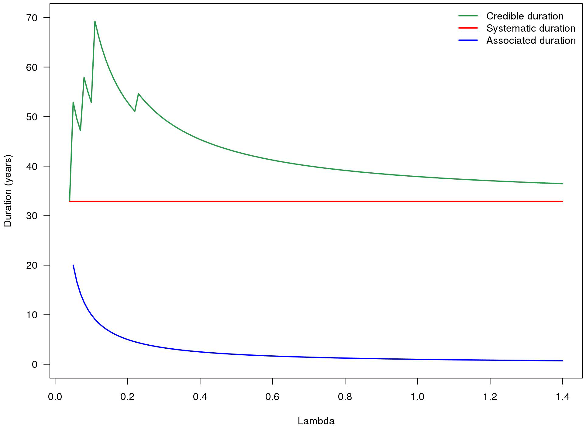
Figure 3 Fictive example of skew surge dataset of systematic and historical data – Credible duration (green line), systematic duration (red line) and associated duration (blue line) for several threshold values.

In conclusion, the sampling threshold choice is an important step in the extreme quantiles estimation allowing the computation of the credible duration. Finally, with all of these elements we can deal with historical data in a regional framework.

4 Application of the FAB method to a real dataset

4.1 Systematic skew surge database and historical data

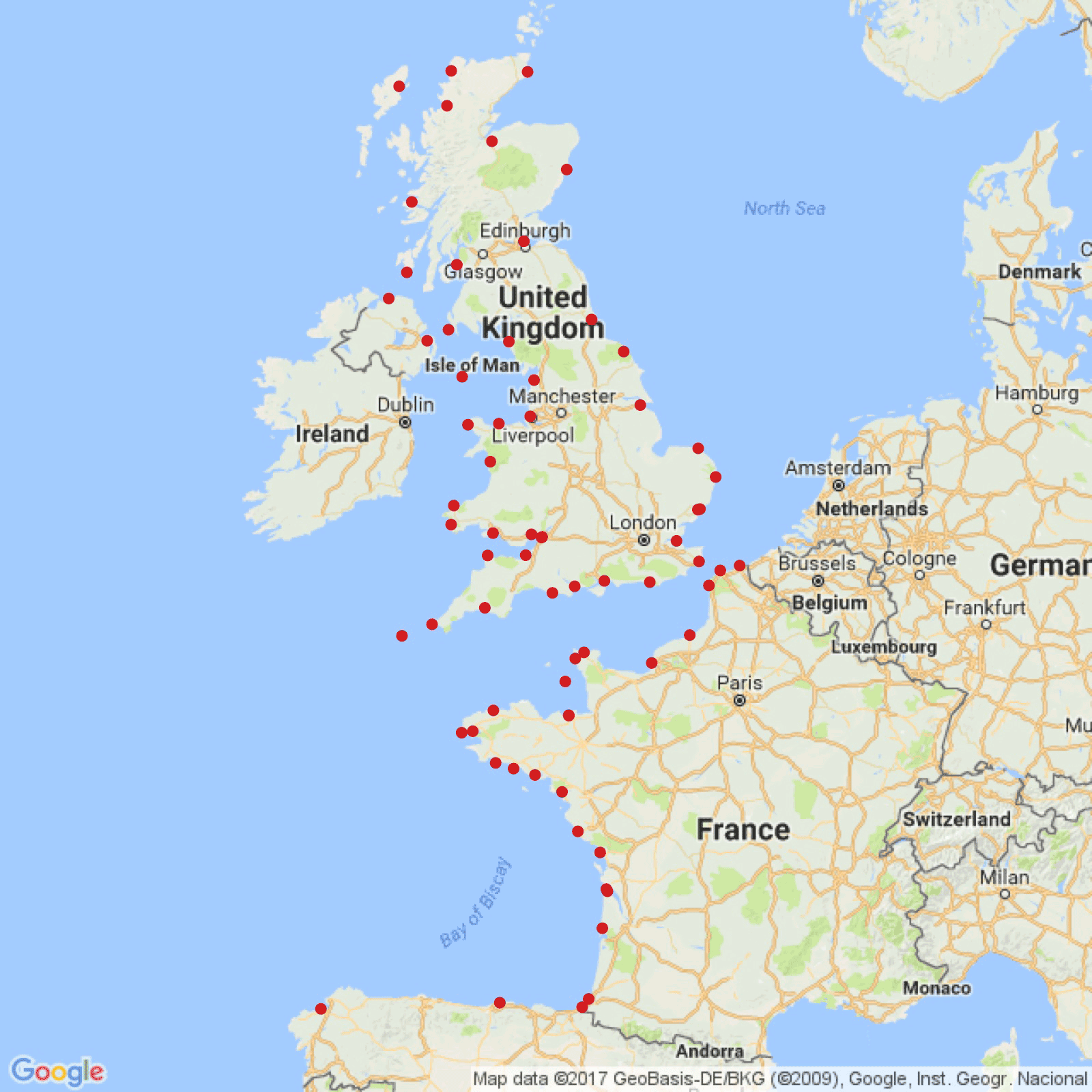
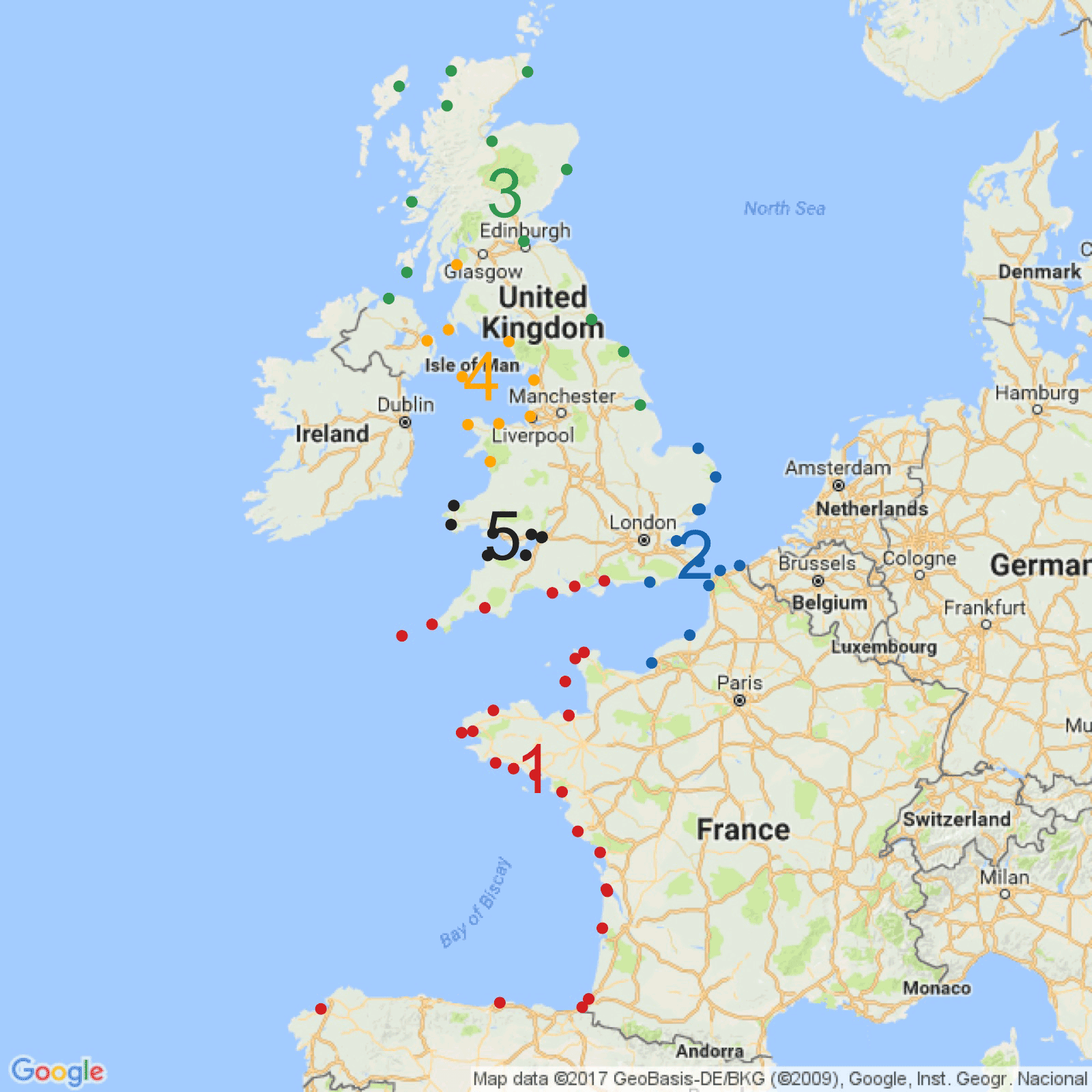
The systematic skew surge database is originated from a time series of sea levels recorded by 71 tide gauges located along French, British and Spanish coasts of the Atlantic Ocean, the English Channel, the North Sea and the Irish Sea (Fig. 4).

French data are provided by SHOM (Service Hydrographique et Océanographique de la Marine, France), English data by BODC (British Oceanographic Data Center, UK) and Spanish data by IEO (Instituto Espanol de Oceanografia, Spain). All data except the Spanish data, are updated to January 2017. Every site has different systematic durations depending on the tide gauge records. Starting from 1846, the longest time series is recorded at Brest for a systematic period of 156.57 years. Sea levels are recorded hourly except for British ports. BODC supplies sea levels every 15 min from 1993 onwards.

Skew surge data are generated at each site from the difference between the maximum sea levels recorded around the time of the predicted astronomical high tide and the self-same predicted astronomical high tide. Before computing skew surge, sea levels must be corrected by a potentially long-term alteration of mean sea levels, or eustatism. Only sea level data with significant linear trends are edited. More details on the computation of skew surges are described by Simon (2007), Bernardara et al. (2011) and Weiss (2014). In this way, the systematic database of 71 skew surge series is created.

Finding accurate historical data is complex and difficult and at the time of writing only 14 historical skew surges are available. These historical records are located in 3 of the 71 ports: 9 at La Rochelle (Gouriou, 2012; Garnier and Surville, 2010; Breilh, 2014; Breilh et al., 2014), 4 at Dunkirk (DREAL, 2009; Parent et al., 2007; Pouvreau, 2008; Maspataud, 2011) and 1 at Dieppe (provided by the Service hydrographique et océanographique de la Marine SHOM, France). The historical data are introduced in corresponding skew surge series of the concerned sites.

This skew surge database of systematic and historical data is exploited in this study for the estimation of regional return periods.

4.2 Formation of regions

The method to form homogeneous regions proposed by Weiss et al. (2014a) is used to get physically and statistically homogeneous regions from the database shown above. This methodology is based on a storm propagation criterion identifying the most typical storms footprints. The configuration of parameters to detect storms is set using the same criteria as Weiss (2014). The most typical storm footprints are revealed by Ward's hierarchical classification (Ward, 1963) and correspond to four physical regions. The homogeneity test (Hosking and Wallis, 1997) is applied to check if all regions are also statistically homogeneous. Only one physical region is not statistically homogeneous, and after an inner partition and a further check, five physically and statistically homogeneous regions are obtained.

Moreover, a double threshold approach (Bernardara et al., 2014) is employed to separate the physical part from the statistical part of the used extreme variables and two different thresholds are used: the first to define physical storms (physical threshold) and the second to define regional samples (statistical sampling threshold, or more simply, sampling threshold).

Figure 5 displays the five regions founded out through the application of Weiss' methodology. Although a different input database is used, the number and the position of the regions are similar to Weiss' study.

The regionalisation process shows that only Region 1 and Region 2 hold historical data. The three sites with historical data belong to these two regions: La Rochelle to Region 1 and Dieppe and Dunkirk to Region 2.

The region with more historical information is the Region 1 (nine historical skew surges) and the results of FAB method proposed are focused on this region.

4.3 Focus on Region 1

4.3.1 Statistical threshold and credible duration

The sample of regional extremes is analysed with statistical tools in order to estimate regional return levels associated with very extreme return periods. A regional pooling method is used to select independent maximum data. A regional sample is formed through normalised local data. Maximum local data are divided by a local index, equal to the local sampling threshold value (Weiss, 2014). Moreover, this methodology enables us to estimate the regional distribution F_r considered as the distribution of the normalised maximum data above the statistical sampling threshold.

This threshold corresponds to a storm's frequency λ, which is assumed equal at all sites of a region. The sampling threshold value selection, or more accurately the λ value selection, is a complicated topic (Bernardara et al., 2014). There is no an unequivocal approach for defining the exact sampling threshold. Twelve sensitivity indicators depending on all possible λ values are proposed to assign the best λ value for the regional analysis of extreme skew surges using historical data: the statistical homogeneity test (Hosking and Wallis, 1997), the stationarity test applied to storm intensities of regional sample (Hosking and Wallis, 1993), the chi-squared test for the regional distribution (Cochran, 1952), the statistical test to detect outliers in regional sample (Barnett and Lewis, 1994; Hubert and Van der Veeken, 2008; Weiss, 2014), the value of regional credible duration, the number of regional sample data, the value of the degree of regional dependence φ, the visual look of the regional return plot and the stability of regional credible duration, local return levels, shape parameter and scale parameter of the GPD distribution (Coles, 2001). The λ value selection can not be carried out through one of these methods and only the combination of all indicators can enable us to appoint the optimal λ. All sensitivity indicators have the same relevance in the proposed sensitivity analysis.

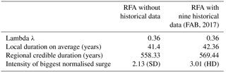
A skew surge's frequency of 0.36 is chosen for Region 1 thanks the sensitivity analysis of the statistical factors mentioned above. Taking λ= 0.36 results in having, on average, one extreme skew surge over the sampling threshold every 2.78 years at each site. This threshold selection permits the computation of the credible duration for every site belonging to the Region 1. In Region 1, all ports except for La Rochelle have only systematic skew surge and their credible duration, equal to systematic duration, is determined and independent from the sampling threshold value.

On the contrary, the site of La Rochelle has nine historical skew surges and its credible duration depends both on systematic duration and historical duration. The systematic duration does not change and it is equal to the recording period of La Rochelle tide gauge. As shown in the fictive illustration of Sect. 3, the historical duration differs as threshold value changes.

The credible duration at La Rochelle is 57.88 years and the contribution of historical data is almost the 43 % of the total duration. Obviously, without these nine historical data, the coverage period of extreme data at La Rochelle would have been less than 25 years, equivalent to the historical duration. All the historical data are over the chosen threshold and, consequently, the associated duration of each historical data is equal to 2.77 years.

Figure 4 Location of the 71 tide gauges used in this study.

Figure 5 The five physically and statistically homogeneous regions of the 71 tide gauges.

4.3.2 Regional credible duration

Equation (11) enables us to compute the regional credible duration for Region 1. The introduction of nine historical data in the local time series and only eight in the regional sample after the use of the regional pooling method, grants an earning of 11.11 years of regional duration. As Table 2 shows, historical data increase the credible durations for sites where there are historical records and consequently the regional credible duration likewise increases. In Region 1, only the site of La Rochelle increases its duration. This contribution allows for the increase of the regional credible duration.

Regional credible duration depends not only on the mean of local duration but also on the degree of regional dependence ϕ (Eq. 11). Obviously, this degree does not change with only nine more added data. In conclusion, the rise of the regional credible duration of Region 1 is produced mostly by the increase of credible duration at La Rochelle.

Table 2 shows the difference with the FAB method that allows to take into account historical data and a traditional method of RFA (Bernardara et al., 2011; Weiss, 2014) that does not enable the use of historical data. Figure 6 displays how the more λ decreases in value, the more the difference between regional credible duration with the nine historical data (blue line) and the regional effective duration without historical data (green line) for Region 1 increases (red line). This is due to the greater certainty that historical data above the sampling threshold are the biggest over a longer period.

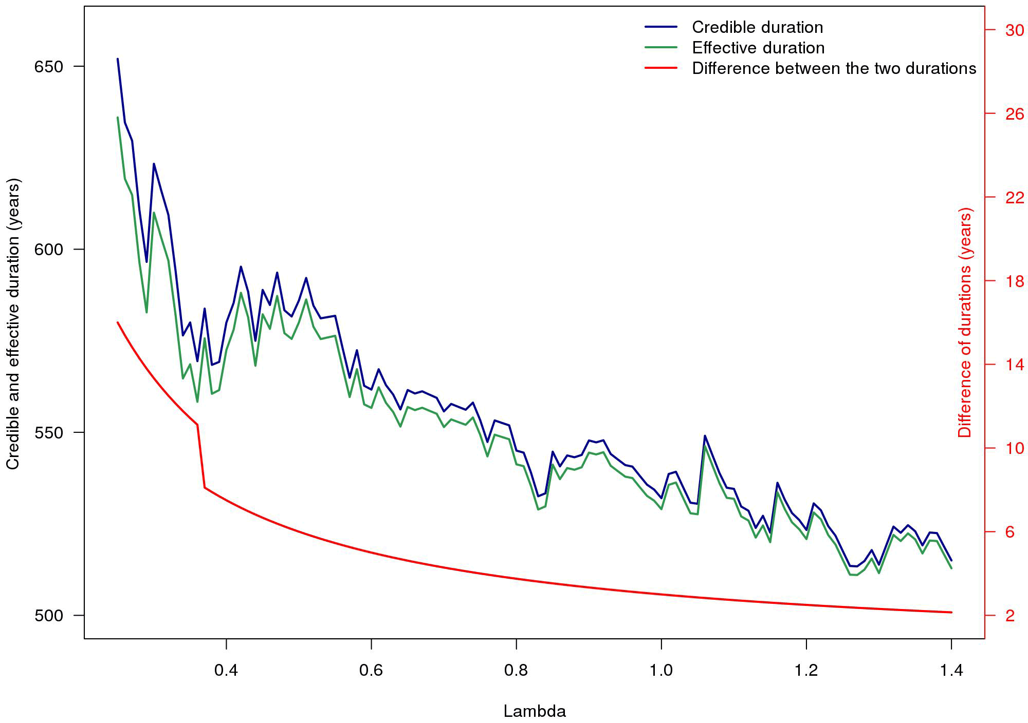
Figure 6 Variation in regional credible duration (taking into account the nine historical data) and regional effective durations (only with systematic data) and their difference (in red) for Region 1.

Table 2 Summary table of the results obtained with the application of FAB method for Region 1.

4.3.3 Regional return levels

Regional return levels for Region 1 are obtained through the fit of a generalised Pareto distribution (Fig. 7). Penalised maximum likelihood estimation (PMLE) (Coles and Dixon, 1999) is used to estimate the regional GPD parameters (γ, k). As shows Fig. 7, the regional distribution is unbounded due to a positive shape parameter k. The return level plot of Region 1 is produced with the 95 % confidence intervals generated by a bootstrap of observed storms. A Weibull plotting position is employed for the regional empirical return period. Return levels for each site are achieved through multiplication between regional return levels and local indices, equivalent to the local sampling threshold.

Red dotted points represent the eight historical data taken into account in Region 1. As it appears, the benefit of using historical data is not only an increase of the coverage period of extreme data but also to be able to consider in a frequency analysis when non-systematic storms occurred. The historical skew surges used in this study represent very big storms and for this reason it is newsworthy to take into account their large magnitude. Indeed, the biggest normalised skew surge considered in Region 1 is 3.01 compared with 2.13 of the regional sample generated without historical data (Table 2).

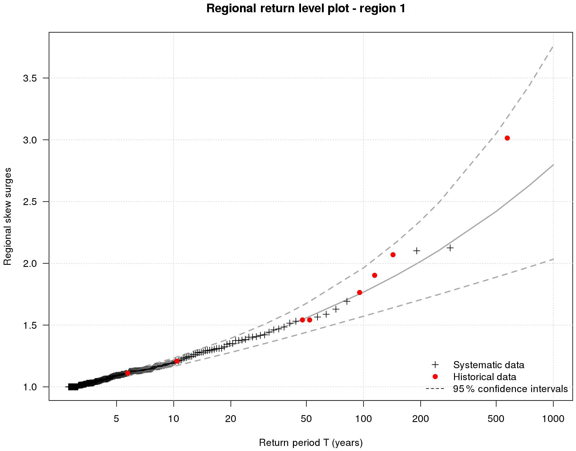
Figure 7 Return level plot for the regional distribution of Region 1 with the confidence intervals of 95 % estimated by bootstrap. Red points represent the regional historical data and black crosses the regional systematic data.

5 Conclusions

The application of the FAB method, based on the new concept of credible duration, allows more reliable extreme estimations of return levels to be obtained due to the inclusion of historical data to a systematic skew surge database.

The introduction of historical data on a frequency analysis of extremes is an innovative way to increase the reliability of estimations. In the past, the estimation of the period covered by the historical data collection has usually limited the use of historical data. The concept of a perception threshold was employed to use historical data even though its hypothesis is quite broad and difficult to verify. For this reason, the new concept of credible duration has been formulated that is based on physical considerations supported by several scientific studies. This leads to use historical isolated data points on the EVA.

The hypothesis, that the frequency of storms λ remains unchanged in time and on which credible duration concept is based, is satisfactory for skew surge. For other variables, a hypothesis check has to be done. Following the hypothesis check, all the considerations that we raised in this study can also be applied for other natural hazards.

When historical data are available, the credible duration depends on sampling threshold. This novelty allows the expansion of the credible duration concept to a regional scale. The RFA is another efficient way to reduce uncertainties on the extreme estimations. These two ways can be used together by the proposed FAB method.

The results describe the relevance of using historical records on a regional analysis both in terms of regional duration and of storm magnitude. Sometimes, these data can represent very large events and so we have to consider them during the estimation of extreme variables. Moreover, the existence of historical records enables to raise the coverage period of the extreme sample.

No extreme data can be missed in an extreme frequency analysis. It is very important to use all of the available data in order to get increasingly more reliable extreme estimations and regional analysis and historical data are two tools that can be merged to get satisfactory results.

New perspectives are opened to improve extreme quantiles estimations by using historical data that is becoming increasingly more available through different investigations on several qualitative and quantitative sources. The aggregation of all of these data in a historical database is a need to exploit the maximum amount of extremes.

Furthermore, every historical data value is associated with different uncertainties and it is challenging to be able to take into account these uncertainties in the regional analysis.