the Creative Commons Attribution 4.0 License.
the Creative Commons Attribution 4.0 License.
 | 21 Feb 2018
Debris flow run-out simulation and analysis using a dynamic model
Theo van Asch
José L. Zêzere
Only two months after a huge forest fire occurred in the upper part of a valley located in central Portugal, several debris flows were triggered by intense rainfall. The event caused infrastructural and economic damage, although no lives were lost. The present research aims to simulate the run-out of two debris flows that occurred during the event as well as to calculate via back-analysis the rheological parameters and the excess rain involved. Thus, a dynamic model was used, which integrates surface runoff, concentrated erosion along the channels, propagation and deposition of flow material. Afterwards, the model was validated using 32 debris flows triggered during the same event that were not considered for calibration. The rheological and entrainment parameters obtained for the most accurate simulation were then used to perform three scenarios of debris flow run-out on the basin scale. The results were confronted with the existing buildings exposed in the study area and the worst-case scenario showed a potential inundation that may affect 345 buildings. In addition, six streams where debris flow occurred in the past and caused material damage and loss of lives were identified.
- Article
(9540 KB) - Full-text XML
- BibTeX
- EndNote


Debris flows are typically initiated by two types of mechanism (e.g., Coussot and Meunier, 1996; Hungr, 2005; Van Asch et al., 2014): (i) infiltration triggered soil slips, which develop into debris flows, and (ii) surface runoff erosion including the entrainment of loose material. The latter is quite common in areas with scarce vegetation, or that have been recently affected by forest fires, thus becoming more susceptible to erosion (e.g., Cannon et al., 2001, 2008, 2011; Cannon and Gartner, 2005,; Santi et al., 2008; Baum and Godt, 2010; Kean et al., 2013; Staley et al., 2013, 2014).
The consumption of vegetation, ash deposition, changes in physical properties of soils and rocks and the presence of water repellent soils are typical consequences of fire (Cannon and Gartner, 2005; Cannon et al., 2010; Parise and Cannon, 2012). In addition, the hydrological response of a burned basin includes the decrease in the infiltration rate and therefore the increase of surface runoff (Cannon, 2001; Cannon and Gartner, 2005; Cannon et al., 2010). Therefore, burned basins are highly susceptible to debris flows, which may be very dangerous for two reasons (Cannon et al., 2011): (i) the amount of rainfall responsible for the triggering of debris flows may be lower when compared to areas that have not been recently affected by wildfires; and (ii) debris flows can be generated in places without past known occurrences.
The development of simulation techniques, especially in recent years, has allowed dynamic modeling to become an increasingly important tool for simulating the characteristics and behavior of debris flows. Nevertheless, knowledge about the initiation mechanisms, erosion and propagation of debris flows is still limited. While most models are focused on the propagation and deposition processes, only a few address the entrainment process and even fewer the initiation mechanism (Van Asch et al., 2014).
The dynamic approach is numerically solved through physically based models based on fluid mechanics. Dynamic continuum models rely on the physical laws of conservation of mass, momentum and energy, and the behavior of the flow material is constrained by its geotechnical properties (Dai et al., 2002; Quan Luna et al., 2012). Some of the rheological models frequently used to characterize the behavior of debris flows are (e.g., Naef et al., 2006; Beguería et al., 2009; Hungr and McDougall, 2009): (1) the Coulomb frictional resistance; (2) the Bingham model; (3) the Coulomb-viscous; and (4) the Voellmy frictional-turbulent resistance.
One of the major challenges of the dynamic approach is to select the most appropriate rheology to simulate the flow behavior as well as to correctly estimate or calibrate the model's key parameters (e.g., O'Brien et al., 1993; Beguería et al., 2009; Hsu et al., 2010; Scheidl et al., 2013). Most frequently, these parameters are estimated by back-analysis of past events (e.g. Naef et al., 2006; Rickenmann et al., 2006; Hürlimann et al., 2008). The calibration by back-analysis is usually performed by trial and error. However, sophisticated automated techniques, like the application of genetic algorithms (e.g. Iovine et al., 2005; D'Ambrosio et al., 2006; Spataro et al., 2008; Terranova et al., 2015) has made it possible to obtain more exhaustive evaluations of the calibration parameters.
Considering that dynamic models rely on physical assumptions, in most cases validation is a complex task. For instance, if the landslide total volume deposited is known, this information can be used for validation purposes (e.g. Van Asch et al., 2014). More often, only scarce information is available and the validation is carried out through the comparison between the spatial pattern of the landslide simulations and the real cases. Frequently, fitness functions (e.g. Iovine et al., 2005; D'Ambrosio et al., 2006; D'Ambrosio and Spataro, 2007; Spataro et al., 2008; Avolio et al., 2013; Lupiano et al., 2015) have been implemented to perform the spatial comparison of real and simulated events.
Consequently, although widely applied on the slope scale, the dynamic approach has been scarcely applied at the medium scale. Regarding the latter, it stands out in the work developed by Revellino et al. (2004) and Hürlimann et al. (2006) that applied one-dimensional numerical models. More recently, Quan Luna et al. (2016) have implemented the “AschFlow”, a two-dimensional one-phase continuum model that simulates the debris flow erosion and deposition processes. In this model, the debris flows are initiated by soil slips and the flow behavior is conditioned by the rheology.
It is worth mentioning other type of dynamic models, for instance based on a discretized viewpoint (e.g. cellular automata), that are suitable to medium and small-scale analysis (e.g. D'Ambrosio et al., 2003; Iovine et al., 2003; Avolio et al., 2011, 2013; Lupiano et al., 2015). Such models integrate the initial soil slip and further material entrainment along the path through a combination of elementary processes, acting within the cells of the computational domain. Despite adopting simplified approaches (e.g. the equivalent fluid), the rheological issues are also taken into account through energy-dissipation options.
In this context, the scarcity of studies applying dynamic models on the basin scale is evident. Thus, the main objectives of the present research are: (1) modeling the run-out of two debris flows triggered during a rainstorm, only two months after a forest fire affected the area; (2) to calculate by back-analysis the rheological and entrainment parameters, as well as the excess rain involved in the triggering of these two debris flows; (3) to apply a two-dimensional one-phase continuum model to estimate the parameters referred in (2). This model simulates the debris flow initiation process by surface runoff, concentrated erosion along the channels, propagation and deposition of flow material; (4) to validate the run-out model using 32 debris flows also triggered in 2005 that were not considered for calibration; and (5) to perform three scenarios of debris flows run-out on the basin scale, using different values of excess rain for each scenario and considering the rheological and entrainment parameters obtained for the most accurate simulation. Scenario results are confronted with the existing buildings exposed in the study area.
The study area is the upper part of the Zêzere valley located in the highest Portuguese mountain range, the Serra da Estrela, in central Portugal (Fig. 1). The elevation ranges from 668 m to 1990 m a.s.l. and gradually decreases from SSW to NNE. The geology is dominantly granitic (Migoń and Vieira, 2014): porphyritic medium- to coarse-grained granite and non-porphyritic medium- to fine-grained granite outcrop over 73 % of the study area. Hornfels constituting a metamorphic aureole are present in the northern part of the study area, whereas the bottom of the valley is covered by Quaternary deposits of fluvial and glacial origin.
In the study area, the effect of weathering on rock strength is mostly evident in coarse and medium granites (Migoń and Vieira, 2014). Migoń and Vieira (2014) ranked the granite types according to their resistance against weathering and erosion as it follows: non-porphyritic medium- to coarse-grained muscovite granite (lithology 8, Fig. 2) > porphyritic medium- to coarse-grained two-mica granite (lithology 6, Fig. 2) > non-porphyritic medium- to fine-grained biotite granite (lithology 9, Fig. 2). According to Migoń and Vieira (2014), lithology 6 is less resistant than lithology 8 especially due to the texture, since the mineralogical composition of both lithologies is similar. The authors also observed, from road cuts in steep slopes, that lithology 9 is deeply weathered. Plus, they refer that this condition is increased by the high biotite content favoring chemical weathering, the presence of magmatic foliation and hydrothermal changes.
The climate is Mediterranean, with warm and dry summers. The mean annual precipitation is circa 2500 mm on the Serra da Estrela (Vieira et al., 2004) and the wet season typically lasts from October to May.
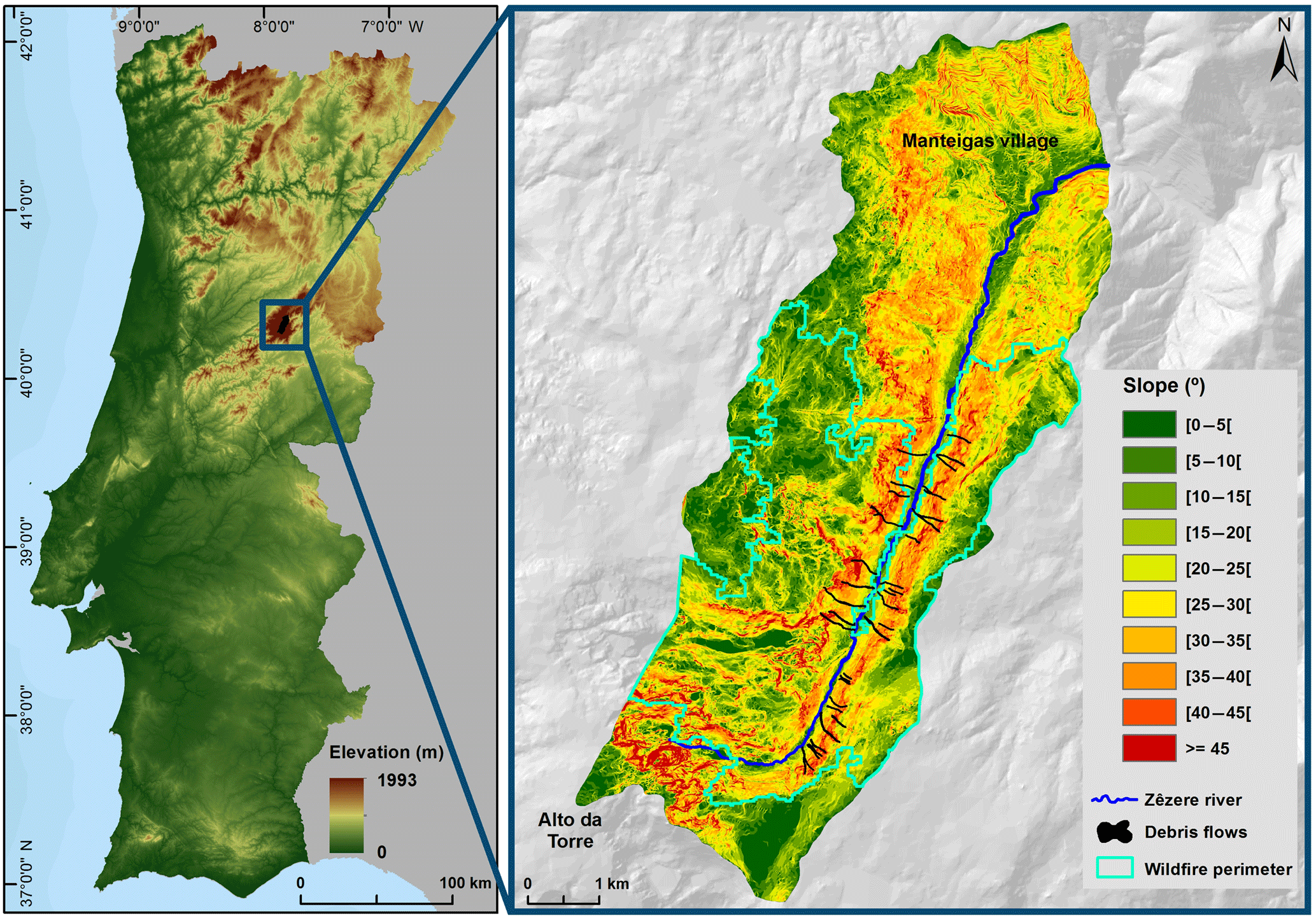
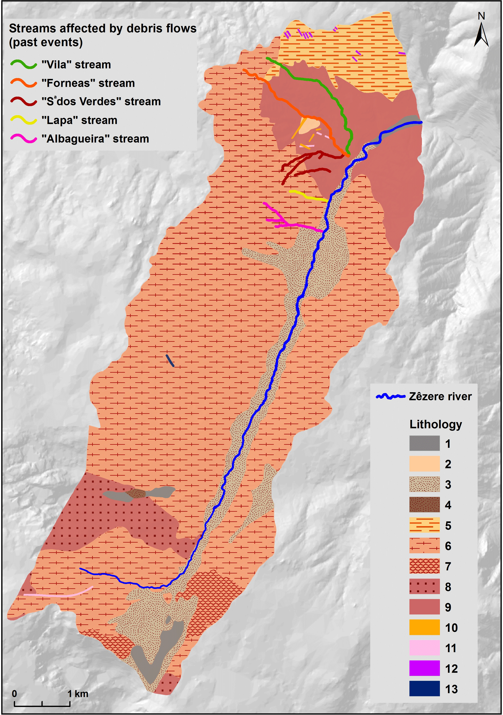
Figure 2Lithology of the study area and streams affected by historical occurrences of debris flows. Lithology: 1 = alluvium; 2 = slope deposits; 3 = fluvioglacial deposits; 4 = glacial deposits; 5 = contact metamorphic rock (hornfels); 6 = porphyritic medium- to coarse-grained two-mica granite; 7 = porphyritic medium-grained two-mica granite; 8 = non-porphyritic medium- to coarse-grained muscovite granite; 9 = non-porphyritic medium- to fine-grained biotite granite; 10 = quartz dikes; 11 = basic rock dikes; 12 = metamorphosed basic dikes; 13 = aplite-pegmatite dikes.
3.1 The event of 30 October 2005 and historical events
During the summer of 2005 a large forest fire burned the southern sector of the study area (Fig. 1) and later, on 30 October 2005, a rainfall triggered debris flow event affected the unprotected slopes. A total of 34 debris flows were identified, most of them along the Eastern slope of the valley (see Fig. 4). Although no victims were registered, the national highway linking the main village to the most touristic places in the higher mountains was closed due to the debris flow occurrence (Melo and Zêzere, 2017). The debris flows were identified and mapped by aerial photo interpretation, analysis of morphological features from post-event topography (1 : 10 000 scale) and systematic field surveying with DGPS during 2011.
The first records on debris flows that occurred in the study area date back to the 19th century. In a particular event, registered in 1804 (along the stream marked in green, in Fig. 2), 20 lives were lost (Melo and Zêzere, 2017). More recently, in 1993 a debris flow occurred in an area burned by a forest fire two years before (along the stream marked in pink in Fig. 2) and produced high material losses for a hotel. The remaining streams, shown in Fig. 2, were also affected by debris flow activity in the past. We think these events are underestimated, especially along the Zêzere valley, due to under-report related to the scarce number of elements at risk. Indeed, there is a lack of quantitative information about debris flows that occurred in the study area. For instance, even for the most recent events, there is no record on the volume of the deposited material or even the total amount of rainfall, although we know it happened after a severe rainstorm.
3.2 Model description
The two-dimensional one-phase continuum model used was developed and applied by Van Asch et al. (2014). The model integrates four components: surface runoff, erosion of loose sediments deposited along the channels, flow propagation and deposition.
It must be kept in mind that physical-based models always need to be adapted to the reality under study. In the research developed by Van Asch et al. (2014), the lack of data about soil type led to the choice of a simple runoff model with a constant infiltration capacity, where the effects of initial moisture content and the sorptivity of the soil are ignored (Eq. 1):
where hr is the excess rain (m s−1) that will feed the surface runoff; i is the rainfall intensity (m s−1); and ks is the soil infiltration capacity (m s−1).
The model integrates the entrainment process through a simple erosion module, which intends to reproduce several mechanisms, such as lateral and vertical erosion, bed destabilization by infiltrating water and undrained loading (Van Asch et al., 2014). The abovementioned processes are related to flow velocity and flow above a critical height, according to the equations suggested by Eglit and Demidov (2005) and McDougall and Hungr (2005) (Eq. 2):
where hsc is the erosion rate (m s−1); β is the erosion factor (m−1); v is the velocity (m s−1); h is the flow height (m); and h* is the critical height for erosion to occur, which is arbitrarily assigned the value of 0.1 m (Van Asch et al., 2014), thus ignoring the soil erosion associated to lower flow height. Given the lack of detailed information about the characteristics of the channels, no distinction is made between the erosion along the channels and along the slopes.
At each time step, the solid material is added to the flow until the maximum volumetric concentration is equal to 0.6. When the volumetric concentration of the solids is below the arbitrary limit of 0.2, the flow velocity is calculated using the Manning's equation (Van Asch et al., 2014) (Eq. 3):
where θ is the slope angle in the direction of the steepest slope; and n is the Manning's coefficient (m s). When the volumetric concentration is higher than 0.2, a simple equation of motion is applied (Van Asch et al., 2014) (Eq. 4):
where g is the gravitational acceleration (m s−2); k is the lateral pressure coefficient; and Sf i the resistance factor, which depends on the flow rheology.
The water and solids are routed separately, obeying the law of mass conservation, and for each time step a new concentration is calculated (Van Asch et al., 2014). To ensure the numerical stability of the model during the simulation, a flexible time step based on the Courant–Friedrichs–Lewy (CFL) condition is used (Beguería et al., 2009). The model is implemented in the PCRaster environmental modeling language (Karssenberg et al., 2001).
3.3 Model setup
The calibration of the model was performed for two debris flows triggered during the event in 2005. These two debris flows (DF#1 and DF#2, see Fig. 4) were selected because of their largest dimension and good preservation in the landscape. Due to the lack of additional quantitative information for calibration (i.e., thickness and volume of the deposits), we considered that the outputs from the model could be valid if they positively answered all the following criteria (Fig. 3): (a) the modeling results must reveal an agreement between the maximum run-out distance simulated and the maximum run-out distance observed; (b) the simulation must mimic the deposition of material, with a few centimeters in thickness, observed along the debris flow transport zone; (c) the maximum absolute thickness of the deposits in the accumulation area must not exceed 3.5 m and the mean value must be between 1.5 and 2.0 m, as we registered during field work. The models were calibrated by trial and error and considered valid if the three predefined criteria are verified. The valid simulations were evaluated by using a fitness function (e.g. D'Ambrosio et al., 2006; D'Ambrosio and Spataro, 2007; Spataro et al., 2008; Avolio et al., 2013) and by calculating the percentage of overlapping area between the simulation results and the real cases. In the fitness function (Eq. 5), R and S are the cells affected by the real and the simulated events, whereas m(R∩S) and m(R∪S) are the measure of their intersection and union.
The fitness function delivers values between 0 and 1. If f(R, S) = 0, it means the real and simulated events do not match, being m(R∩S) = 0. On the other hand, if f(R, S) = 1, the real and simulated events are perfectly overlapped, being m(R∩S) = m(R∪S). Values greater than 0.7 are acceptable for two dimensions (Lupiano et al., 2015).
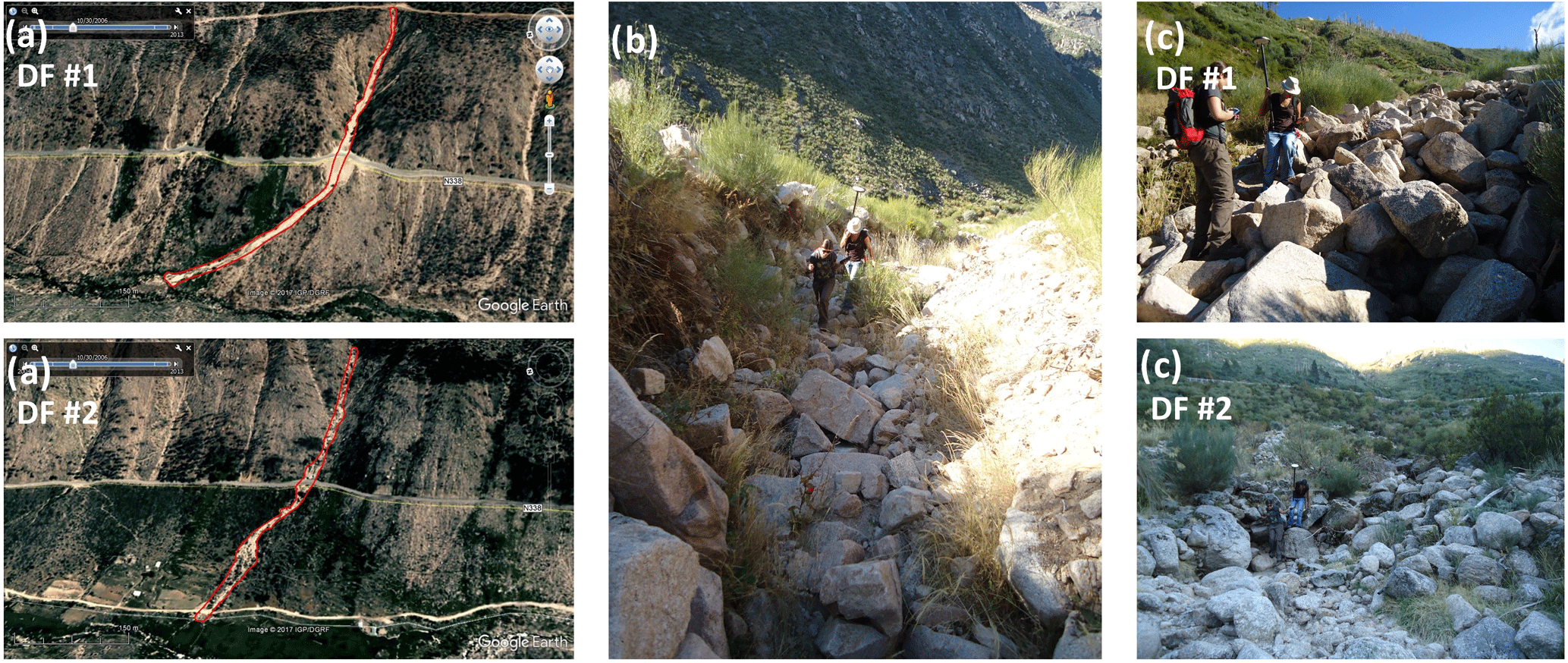
Figure 3(a) Debris flow identification and delimitation; (b) material deposited in the transport zone; (c) deposits in the accumulation area.
After calibration, the model was validated using the remaining 32 debris flows triggered in 2005 that were not considered for calibration (see Fig. 4). The validation included the estimation of the overlapping area between the simulation results and the real cases, as well as the fitness function obtained for each simulated vs. real debris flow.
3.3.1 Rain duration and excess rain values
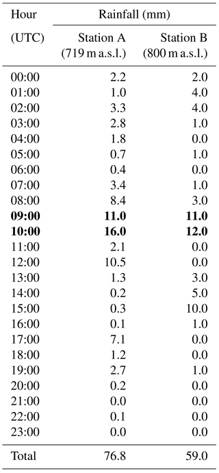
The duration and amount of rainfall involved in the triggering of debris flows are of major importance for the run-out assessment using a dynamic model. It is also known that rainfall hourly data are more important than rainfall cumulative daily data for the triggering of shallow landslides and for the development of hydraulic processes on the slopes. For instance, Malet and Remaître (2011, in Van Westen et al., 2014) found that debris flows are generally triggered by storms lasting from 1 to 9 h. However, there is no information about the duration or the total amount of rainfall occurred on the mountain, where the debris flows were triggered. Nevertheless, the two nearby rain gauge stations registered a 2 h period with the highest values of rainfall (Table 1). Although the two stations are located at distinct topographic positions and several kilometers away from the place where the debris flows occurred (Station A is located at the bottom of the mountain and Station B is in Manteigas village), the models were computed considering a rain duration of 2 h, since we do not have more precise information.

Figure 4Digital elevation model (DEM) of the study area and debris flows that occurred in 2005.
The lack of information on the amount of rainfall and on detailed characteristics of the soils in the study area is a major drawback for proper dynamic model application. To overcome this limiting issue, we chose to calibrate the model based on the excess rain values, which means the amount of water that will feed the surface runoff once the infiltration is exceeded. Thus, surface runoff reflects not only the total rainfall, but also the interaction between rainfall and the soil system.
3.3.2 Rheology and erosion coefficient
The calibration of the geotechnical parameters was performed using four different rheological models: (1) the Coulomb frictional resistance; (2) the Bingham model; (3) the Coulomb-viscous; and (4) the Voellmy frictional-turbulent resistance.
Table 1Rainfall registered on 30 October 2005 at the two rain gauge stations near the Zêzere valley. Stations A and B are located at a linear distance of ca. 8 and 8.5 km from the path of the debris flows, respectively. Bold values indicate the 2 h period with the highest values of rainfall.
The Coulomb frictional resistance is based on the relationship between the effective bed and normal stress at the base of the flow and the pore fluid pressure (Hungr and McDougall, 2009; Ferrari et al., 2014):
where Sf is the unit base resistance; ru is the pore-pressure ratio (–); and φ (∘) is the dynamic basal friction angle. The basal stress is frictional if ru is considered constant, which means that the total normal stress and the shear stress remain proportional. Thus, the equation can be simplified by only including the basal friction angle.
The Bingham model assumes that the debris flow material exhibits a visco-plastic behavior, with laminar flow. The basal shear stress is calculated using Eq. (7) (Beguería et al., 2009):
where Sf (–) is the unit base resistance; ρgh is the normal stress – ρ is the mass density (kg m−3) of the flow and g (m s−2) is the gravitational acceleration –; τc (kPa) is the constant yield strength due to cohesion; η (kPa s) is the dynamic viscosity; h (m) is the thickness of the flow; and v (m s−1) is the flow velocity.
Since debris flows are often composed of sediments with different sizes, one way of considering the friction effect resulting from contact between particles is to complement the Bingham model with the Coulomb's friction resistance component (De Blasio, 2011). Thus, Johnson (1970, in De Blasio, 2011, among others) modified the Bingham model by incorporating the frictional resistance component, which led to the development of Coulomb-viscous model, whose application extends to a wider range of fluids. In this model (Eq. 8), the yield strength results from the combination of cohesion and friction forces (Beguería et al., 2009):
The Voellmy model was initially applied to the simulation of snow avalanches (Voellmy, 1955 in Ferrari et al., 2014) but ever since has been used for modeling landslides of granular material, cohesionless, with or without interstitial fluid (Ferrari et al., 2014) and with turbulent behavior. The model combines a basal friction coefficient similar to Coulomb's apparent friction (φ′) and a resistance term (turbulent coefficient, ξ) similar to the Chézy resistance for turbulent water flows in open channels. The basal shear stress is given by Eq. (9) (Ferrari et al., 2014):
where ξ (m s−2) is the turbulent coefficient.
The range of values selected to represent the cohesion, the viscosity and the turbulent coefficient were taken from a compilation of studies carried out by Quan Luna (2012) about debris flows occurred in a similar geological context, namely in decomposed granites.
The erosion coefficient was calibrated according to the modeling results.
3.3.3 Constant parameters
In addition, the model requires the input of information (related to maps and some model parameters), which was considered constant during the calibration of the excess rain, rheology and erosion coefficient, namely:
- a.
digital elevation model (DEM)
- b.
soil thickness
- c.
Manning's n (= 0.04)
- d.
lateral pressure coefficient (= 1)
- e.
gravitational acceleration (= 9.8 m s−2)
- f.
unit weight of water (= 9.8 kN m−3)
- g.
unit weight of the debris flow (decomposed granite + water = 19 kN m−3)
- h.
unit weight of the bed material (solid granite = 26 kN m−3)
3.4 Modeling the debris flow run-out on the basin scale using the two-dimensional one-phase continuum model
The use of a dynamic model to simulate the debris flow run-out on the basin scale is a major objective of this work. To achieve this purpose, three different scenarios were created based on the combination of excess rain values, erosion coefficient and rheological parameters that best reproduced the two major debris flows occurred in 2005. However, it is necessary to keep in mind that these parameters – not only the precipitation, and consequently the surface runoff, but also the rheology – most certainly vary over the basin. Thus, the creation of scenarios aims to address the following question: what would be the response of the basin if a certain value of excess rain occurred, considering the rheological parameters and the erosion coefficient that best reproduced the run-out of the two major debris flows triggered during the 2005 event? To answer this question, we developed three scenarios (A–C), with excess rain values of 30, 35 and 40 mm h−1, respectively.
The two maps used as inputs for the model are: (1) a DEM with 5 m resolution, which reflects the topography prior to the debris flows occurrence (Fig. 4); and (2) a map of the soil thickness – interpreted as the depth to bedrock – based on the simplified geomorphologically indexed soil thickness (sGIST) model (Catani et al., 2010; Segoni et al., 2012) (Fig. 5). The latter was validated by comparing the results with 38 field point measures, resulting in a mean absolute error of 29 cm (Melo and Zêzere, 2017). It is important to emphasize the numerical and spatial limitation of these data. However, it is very difficult to find cuts in natural slopes along the study area, since most of them involved some kind of anthropogenic intervention (mainly for road construction).
The calibration of the rheology and the erosion coefficient are only performed after a minimum value of excess rain with capacity to trigger debris flows is determined for the study area. This excess rain threshold was calibrated by manually assigning an initial low value and, based on the modeling results, increasing it (using and amplitude of 1 mm h−1) until excess rain capable to trigger debris flows was found. The trial and error calibration demonstrated that excess rain values lower than 28 mm h−1 are not enough to mobilize the loose sediments available on the slopes of the study area. By increasing 1 mm h−1 of excess rain at each model simulation we found out that values above 30 mm h−1 are required for sediment mobilization in DF#1 and DF#2. Regarding the modeling results for the two debris flows (DF#1 and DF#2, see Fig. 3), the trial and error calibration have shown that DF#1 requires excess rain of 32 mm h−1 to allow the calibration of the rheology and the erosion factor, since lower values result in insufficient deposit thickness and insufficient run-out distances, despite the variation of the previously mentioned parameters. For the same reasons, DF#2 requires excess rain of 33 mm h−1 to allow the calibration of the rheology and the erosion factor.
As already referred, the range of values selected to calibrate the cohesion, the viscosity and the turbulent coefficient were taken from a compilation of studies carried out by Quan Luna (2012). The cohesion was calibrated using values between 0.8 and 1.0 kPa (with a range of 0.1 kPa). For the calibration of viscosity, we also used values between 0.8 and 1.0 kPa s (with a range of 0.1 kPa s). In the Voellmy model, the values used for the turbulent coefficient vary between 400 and 2000 m s−2 (with a range of 200 m s−2). Concerning the apparent friction angle, we choose the values of 9, 14 and 21∘ which correspond to the minimum, medium and maximum values used in the studies compiled by Quan Luna (2012). The selection of only three values of apparent friction angle was intentional, to reduce the number of computed simulations. Regarding the erosion coefficient, values between 0.0010 and 0.0014 m (with a range of 0.0001 m) were tested.
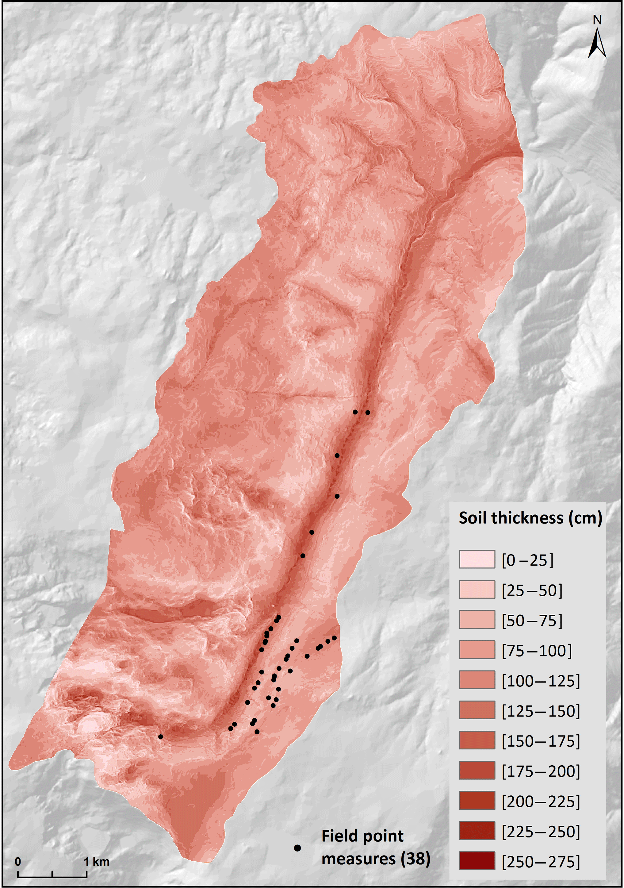
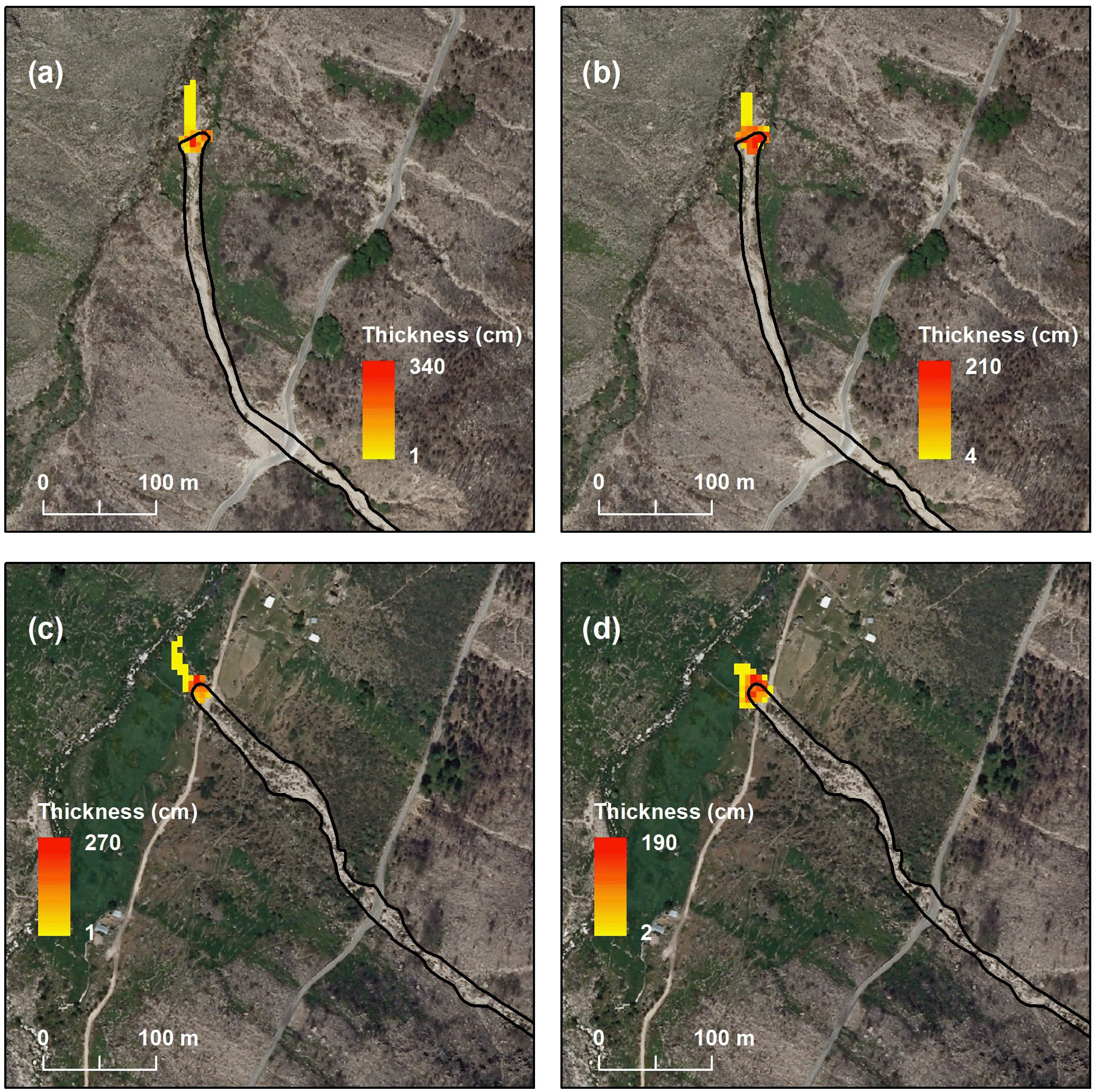
Figure 6DF#1 and DF#2 modeling with the Coulomb frictional (a, c) and with the Voellmy (b, d) models.
Table 2Statistical summary for the 180 simulations performed with Bingham and Coulomb-viscous models for DF#1.
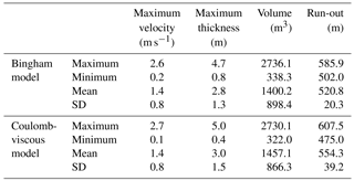
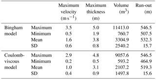
Table 3Statistical summary for the 180 simulations performed with Bingham and Coulomb-viscous models for DF#2.
Considering the validation criteria previously defined, the model versions using the Coulomb frictional and the Voellmy frictional-turbulent resistance were excluded. Looking at some modeling results (Fig. 6), it is clear that both rheologies originate a material deposition only in the most distal part of the debris flows, which means the models are unable to reproduce the deposition observed along the transport zone.
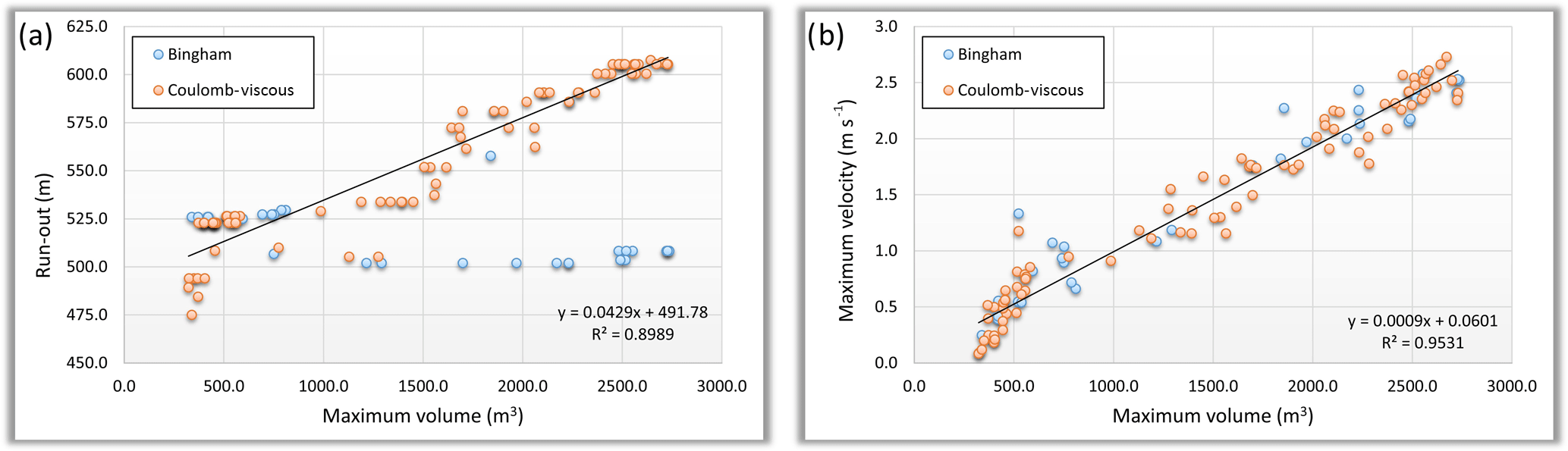
Figure 7Correlation between the maximum volume and (a) the run-out and (b) the maximum flow velocity, for DF#1.
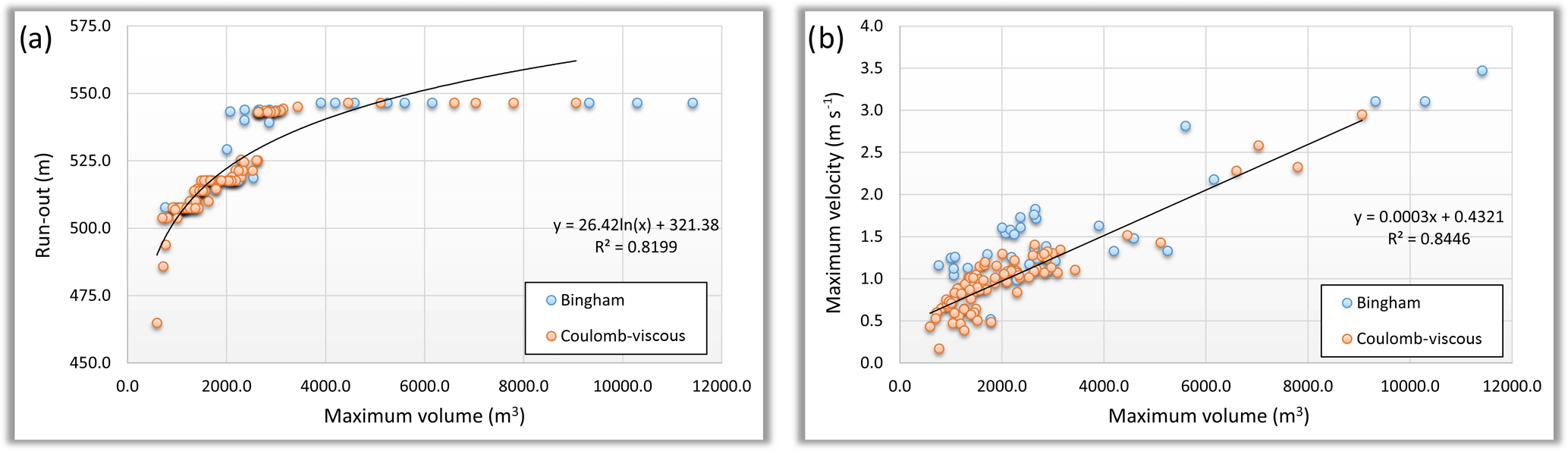
Figure 8Correlation between the maximum volume and (a) the run-out and (b) the maximum flow velocity, for DF#2.
Table 4Parameters used and estimations obtained for the most accurate simulations.
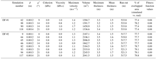

Figure 9Temporal evolution of deposited material thickness, considering a simulation whose results agree with all three predefined criteria (Model run #62 for DF#1 and Model run #64 for DF#2).
The simulations performed with the Bingham and Coulomb-viscous models do not present the abovementioned limitation. Tables 2 and 3 show the statistical summary for the 180 simulations performed with Bingham and Coulomb-viscous models for DF#1 and DF#2. In general, both models apparently produce very similar results. Regarding DF#1, the main differences are related to the run-out, whose values are higher with the Coulomb-viscous model. In relation to DF#2, the differences produced by both models are slightly more pronounced, standing out the maximum volume and the minimum run-out obtained with the Bingham model. In order to understand if there is a relation between some of the most important parameters that reflect the magnitude and intensity of debris flows, correlations between the maximum volume and the run-out, as well as the maximum volume and the maximum flow velocity are analyzed, considering the results obtained with both Bingham and Coulomb-viscous models. The correlations established are summarized in Figs. 7 and 8. DF#1 presents a strong positive linear correlation between the maximum volume and the run-out (a) and the maximum flow velocity (b) (R2 = 0.90 and R2 = 0.95, respectively) (Fig. 7). However, considering the relation between the maximum volume and the run-out, we can detect a few outliers in the results with Bingham model (Fig. 7a). These outliers represent simulations that produced similar volumes but shorter run-outs, in comparison with the simulations performed with the Coulomb-viscous model, despite the same values of cohesion, viscosity and erosion coefficient were used. The R2 estimated for the correlation between the maximum volume and the maximum flow velocity (Fig. 7b) indicates a strong positive linear correlation (R2 = 0.95), without major differences between the two rheological models. Regarding DF#2, the logarithmic function is the one that best describes the relation between the maximum volume and the run-out (Fig. 8a), with a high coefficient of determination (R2 = 0.82). However, for the same run-out, higher volumes are observed with Bingham rheology. The relation between the maximum volume and the maximum flow velocity (Fig. 8b) is best represented by a positive linear correlation (R2 = 0.84). The maximum velocities obtained are slightly higher when the Bingham rheology is used.
Considering that the previously analyzed models represent the material deposition along the transport zone, it must be verified if the other two criteria are also valid, namely the thickness observed in the accumulation area and the agreement between the maximum run-out distance simulated and the maximum run-out distance observed. The overall selection accounted 1 simulation with the Bingham model and 11 simulations with the Coulomb-viscous model that had positively answered these two validation criteria.
Table 4 shows the combination of rheological parameters and erosion coefficient, as well as the maximum flow velocity, deposit thickness, volume and run-out estimated for the 12 most accurate models (the models computed for DF#1 are highlighted in blue and for DF#2 in orange). The debris flow run-out was estimated based on the distance between the initiation and the most distal position of the deposited material. The real run-out of DF#1 and DF#2 is respectively 521.8 and 498.9 m. The maximum and the mean thickness of the deposits, as well as the volume, are slightly higher for DF#2, though the velocity is lower. Regarding the run-out distances, the mean values vary 12 m from the real one for DF#1 and 20 m for DF#2. However, we highlight that the maximum run-out distance was delimited considering the abrupt terminal lobes, composed of coarse material, whose deposits tend to remain preserved. Frequently, the head of the debris flow is overcome by the thin, saturated debris that constitute the body and the tail of the flow. Therefore in this case, since the field surveying was carried out six years after the event took place, it is possible that the real run-out distance was underestimated. The evaluation of the 12 most accurate models (Table 4) demonstrates that in every single case the overlapping area between the simulation and the real case is above 77 %. Furthermore, the fitness function values obtained in all the simulations considered show a good spatial agreement between the modeling results and the real debris flows.
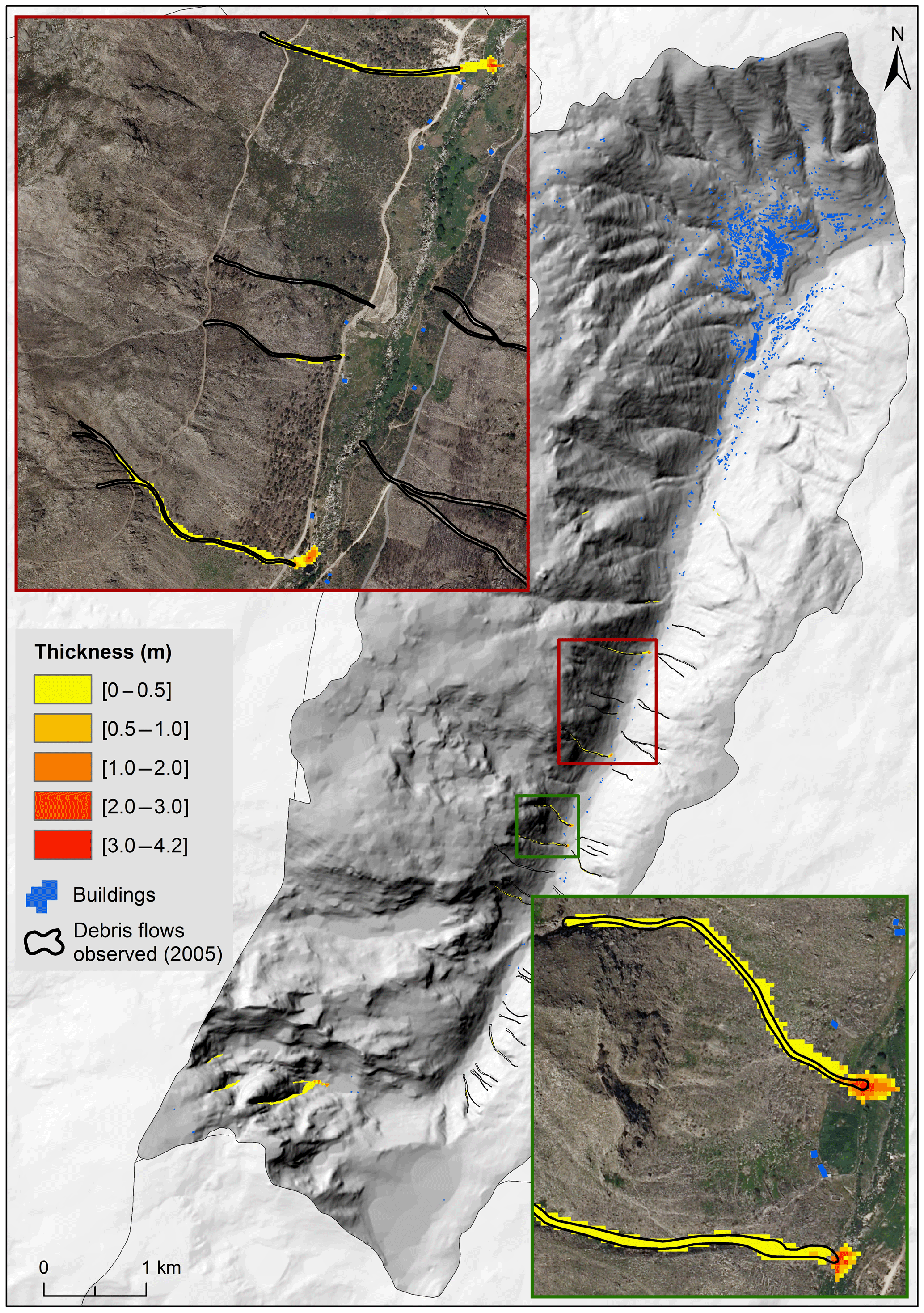
Figure 10Debris flow run-out modeling on the basin scale, considering excess rain of 30 mm h−1 (Scenario A).
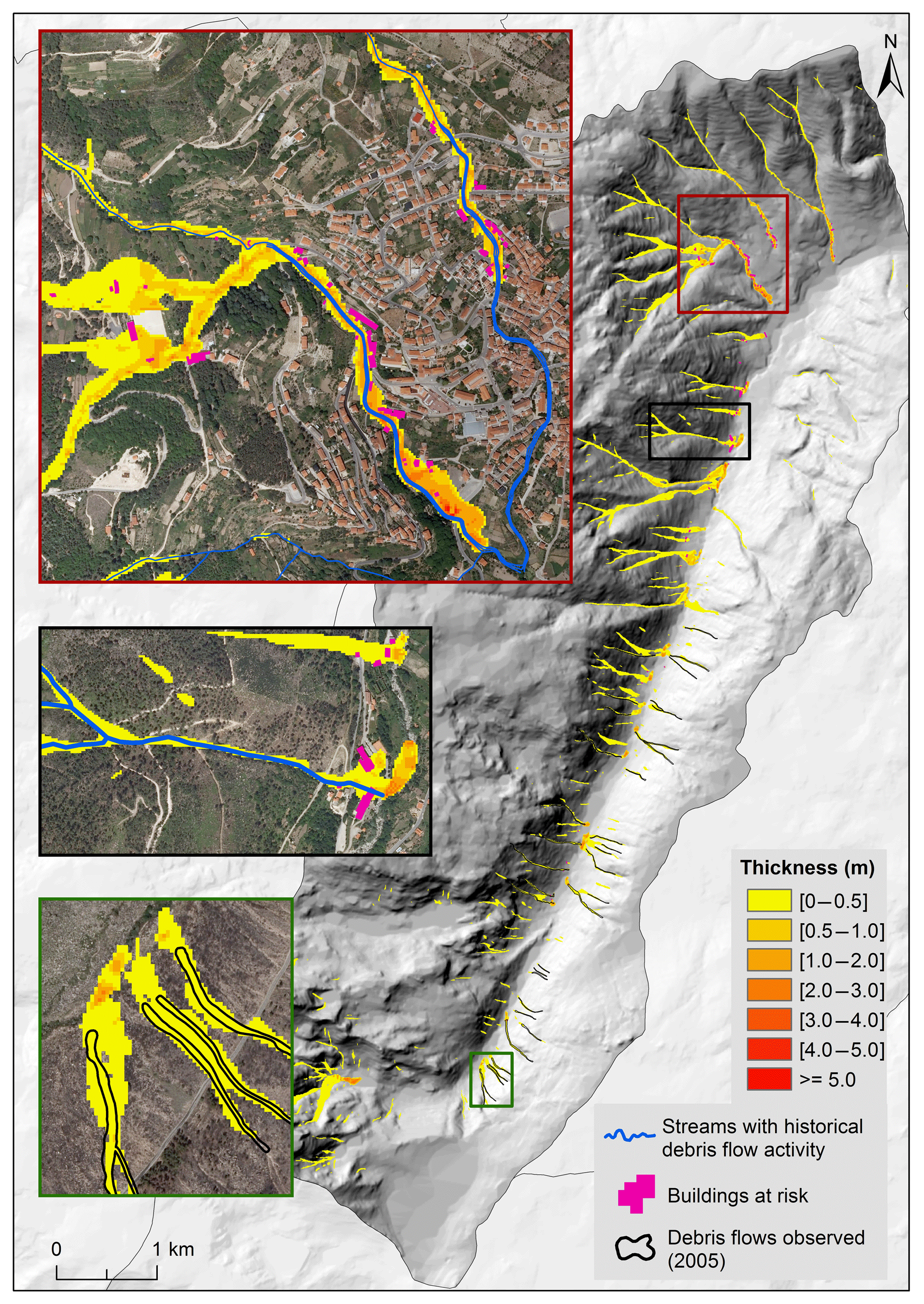
Figure 11Debris flow run-out modeling on the basin scale, considering excess rain of 35 mm h−1 (Scenario B).
Figure 9 shows the temporal evolution of the deposited material thickness, considering a simulation whose results agree with all the three predefined criteria (Model run #62 for DF#1 and Model run #64 for DF#2). Compared to static models, the dynamic models have the advantage of allowing the simulation of the evolution in space and time of a given process. For example, the model application returns a duration of 53 min for DF#1 and 77 min for DF#2, considering debris flows initiation, transport and deposition stages.
The ability of the models computed with 32 and 33 mm h−1 of excess rain (during a period of 2 h) was validated for the remaining 32 debris flows triggered in 2005, and not considered for calibration, and these results are summarized in Table 5. Concerning the modeling computed with excess rain value of 32 mm h−1, the mean percentage and the standard deviation of the overlapped areas (simulated vs real) is ca. 50.2 and 37.5 %, respectively. When excess rain of 33 mm h−1 is considered, the mean percentage increases (67.7 %) whereas the standard deviation slightly decreases (30.2 %). The fitness function validation calculated for the simulation using excess rain of 32 mm h−1 shows that 50 % of the debris flows have values above 0.7. If we consider excess rain of 33 mm h−1, 78 % of the debris flows have values above the referred threshold.
After validation, the debris flow run-out was simulated for the complete study area, considering three different scenarios of excess rain (30, 35 and 40 mm h−1), during a period of 2 h. The values assigned to the rheological parameters, as well as to the erosion coefficient, were based on the arithmetic mean obtained for the 12 most accurate simulations (shown in Table 4): φ′ = 14∘; cohesion = 0.9 kPa; viscosity = 0.9 kPa s; and β = 0.0013 m.
Figures 10–12 show the modeling results for scenarios A–C with excess rain values of 30, 35 and 40 mm h−1, respectively. Table 6 summarizes the maximum velocity, maximum thickness, total volume and maximum run-out obtained for the three scenarios.
In Scenario A (Fig. 10) the debris flows achieve a maximum velocity of 3.5 m s−1 and a maximum thickness of 4.2 m. Table 7 shows that 1 % of the deposits have thicknesses equal or above 2 m. The overlay between the existing buildings and the modeling result shows that there are no buildings at risk. Moreover, as it can be seen in the enlarged frames in Fig. 10, only 5 out of the 34 debris flows triggered during the 2005 event were reproduced, which means the excess rain value used in this scenario (30 mm h−1) is not high enough to mobilize the sediments along the gullies where most debris flows occurred in 2005.
Table 5Validation of 32 debris flows (not used for calibration) considering the modeling results using 32 and 33 mm h−1 of excess rain.
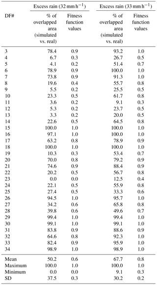

Figure 12Debris flow run-out modeling on the basin scale, considering excess rain of 40 mm h−1 (Scenario C).
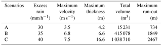
Table 7Classification of the deposits thickness and occupied area (Scenario A).
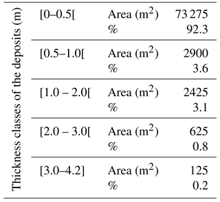
Table 8Classification of the deposits thickness and occupied area (Scenario B).
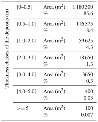
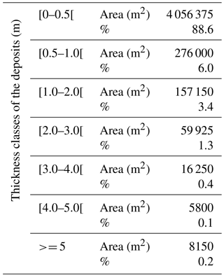
Table 9Classification of the deposits thickness and occupied area (Scenario C).
Concerning the Scenario B (Fig. 11), where excess rain of 35 mm h−1 was used, the debris flows achieve a maximum velocity of 6.8 m s and a maximum thickness of 6.6 m. In this scenario, 1.6 % of the deposits have thicknesses equal or above 2 m (Table 8). The overlay between the existing buildings and the simulation result accounts for a total of 116 buildings at risk. With the Scenario B, all the 34 debris flows triggered during the 2005 event were reproduced in the simulation. This is not entirely legible in Fig. 11 due to the overlay between the debris flows and the simulation result, but the frame (with green outline) shows an example. The total amount of debris flows simulated in this scenario surpasses the event of 2005, which means the latter must lie between scenarios A and B. In addition, by comparing the modeling result with Fig. 2, it is clear that Scenario B is able to simulate the material deposition in 4 streams with historical reports of debris flow activity in the study area. In Fig. 11, the two frames outlined in black and red show the overlay between the streams with historical debris flow activity and the modeling result. The red frame shows the stream where the deadliest debris flow, known to date in the study area, took place killing around 20 persons and destroying a same number of houses. Considering the simulation result we can, nowadays, account for 35 buildings at risk only in this stream. The black frame shows the stream in which was triggered the debris flow that affected a hotel in 1993. In this more recent event, eyewitnesses recalled debris deposits of about 1 m against a wall of the hotel on the ground floor. In Scenario B, this hotel is also affected by a debris flow, but the model simulates a maximum flow thickness of 0.6 m. However, it must be kept in mind that the model is not considering any kind of obstacles that are not covered by the DEM.
Finally, Scenario C (Fig. 12), where excess rain of 40 mm h−1 was used, was considered the worst-case scenario of this study. Here, 2 % of the deposits have thicknesses equal or above 2 m (Table 9) and we can also account for 345 buildings at risk. Moreover, this scenario is able to simulate the material deposition in all the 6 streams identified with historical debris flow activity in the study area.
The model was implemented in the PCRaster environmental modeling language, which runs on Linux and Windows. Concerning this work, we used a computer with a i3 2.13 GHz processor and 4 GB of RAM (64-bit operating system). Under these system specifications, the debris flows simulation on the basin scale (over 44 km2) took ca. 72 h to be completed. Although a faster performance can be obtained using more powerful machines, this dynamic model is currently inappropriate for use as a real-time early warning system. Even a better computational time would unlikely surpass the gap between the rainfall event and the occurrence of debris flows initiated by surface runoff. In this study we used the excess rain values to calibrate the model given the lack of information about the rainfall amount and the soils in the catchments. This option is a good first approach to define hazardous areas, as well as the maximum volume and velocity reached by debris flows. Whenever a nearby rain gauge is available, a deeper investigation about the characteristics of the soils should be considered, at least on the most hazardous sites, in order to use the hydraulic conductivity values to develop a wide range of scenarios on the basin scale using different precipitation inputs. In case of imminent risk, the most suitable scenario can be chosen according to the amount of rainfall at that time. This information can be immediately directed to civil protection and first-response emergency services.
In this work, we applied a two-dimensional one-phase continuum model to calibrate by back-analysis, the excess rain involved, as well as the rheological parameters that best reproduced the two major debris flows triggered during an intense rainstorm in 2005, only two months after the area was burned by a huge forest fire.
The model applied simulates the debris flow initiation process by surface runoff, the erosion, the flow propagation and the deposition of the traveled material, which means the model is suitable to simulate debris-flows in recently burned areas, considering the main initiation mechanism is due to runoff erosion. Moreover, the erosion module allows the simulation of the volume increase due to material entrainment. The rheological parameters and the erosion coefficient that produced the best simulations were validated using 32 debris flows not considered for calibration, and were used to compute a debris flow run-out modeling on the basin scale. Three scenarios were elaborated using different excess rain values and, for each scenario, the buildings at risk were accounted.
The debris flow run-out modeling using a physically based model presents several advantages when compared with the most common data-driven models. Unlike the latter, physically based approach allows for the estimation of flow velocities, thickness of the deposits and impact force against obstacles. Such parameters are of paramount importance for the development of warning systems and structural mitigation measures. In addition, this type of model is not dependent on local conditions and do not require landslide inventories for modeling procedures, which is an advantage when the modeling is performed for locations where no inventories are available. Nonetheless, such inventories may remain essential to calibrate the rheological parameters by back-analysis and for validation purposes (Oliveira et al., 2017).
On the other hand, the reliability of the modeling results is strictly dependent on the DEM and the soil thickness map. When the modeling intends to reproduce an event that occurred in a certain catchment, the DEM must represent the topography prior to the event. In addition, the soil thickness must be estimated for the entire catchment, which is not an easy task. The difficulty in estimating the spatial variation of this parameter frequently leads to the use of a constant value. However, this is not advisable when the model is computed on the catchment scale and if the primary debris flow initiation mechanism is due to runoff erosion, unlike the located infiltration triggered soil slips that develop afterwards into debris flows. If more precise information exists for the study area, namely the characteristics of the soils in the catchments and the hourly total amount of rainfall obtained near the sites of debris flow development, the model would use these parameters instead of being calibrated based on excess rain. This would allow estimating critical rainfall thresholds for the study area (Van Asch et al., 2014). In addition, further information on initiation-track-deposition zones of real cases, on the depth of erosion due to entrainment, the thickness of deposits, and the velocities attained by real debris flows would reduce the uncertainty of all assumptions that were made when assigning the model parameters and would significantly increase the reliability of calibration and validation of the model.
As already highlighted by Quan Luna et al. (2016), the integration of different rheological models allows the comparison of the different results. This provides a flexible choice for the user, not only regarding the scenario that best reproduces the event occurred, but also concerning the use of the rheology most adequate to the type of event under analysis (e.g., hyperconcentrated or granular), which is a major advantage for the development of future scenarios.
The work developed also intends to show the importance of dynamic modeling for the debris flow run-out assessment. The output of the model allowed the calculation of flow velocity, thickness of the deposits, volume and extent of traveled material, on the basin scale. These are extremely important parameters that should be considered in further studies on hazard and risk assessment.
Despite many uncertainties, another advantage of dynamic modeling is the possibility to bring in the temporal component for a hazard analysis for debris flows at the regional scale. Running scenario's with different intensities of rain events, which have different return periods, enables one to distinguish areas at risk, with different temporal frequencies and impact intensities. This can provide important information for cost benefit analyses and mitigation planning.
The code is not publicly accessible because it is currently being used for further investigation within an ongoing PhD thesis.
RM, TWJvA and JLZ conceptualized the study. TWJvA developed the dynamic model and contributed to its adaptation to the study area. RM and JLZ performed field work. RM prepared the data, the models and the manuscript with contributions from all authors.
The authors declare that they have no conflict of interest.
This article is part of the special issue “Landslide early warning systems: monitoring systems, rainfall thresholds, warning models, performance evaluation and risk perception”. It does not belong to a conference.
This work was financed by national funds through FCT – Portuguese Foundation for Science and Technology, I.P., under the framework of the project FORLAND – Hydro-geomorphologic risk in Portugal: driving forces and application for land use planning (PTDC/ATPGEO/1660/2014). Topography data courtesy of the Manteigas Municipality.
We acknowledge the editor of the special issue and two anonymous reviewers
whose pertinent comments and suggestions helped to improve the quality of the
work.
Edited by: Stefano Luigi Gariano
Reviewed by: Giulio G. R. Iovine and one anonymous referee
Avolio, M. V., Bozzano, F., D'Ambrosio, D., Di Gregorio, S., Lupiano, V., Mazzanti, P., Rongo, R., and Spataro, W.: Debris flows simulation by cellular automata: a short review of the SCIDDICA models, in: 5th International Conference on Debris-Flow Hazards Mitigation, Mechanics, Prediction and Assessment, IJEGE book, edited by: Genevois, R., Hamilton, D. L., and Prestininzi, A., Casa Editrice Università La Sapienza, Rome, Italy, 387–397, 2011.
Avolio, M. V., Di Gregorio, S., Lupiano, V., and Mazzanti, P.: SCIDDICA-SS3: a new version of cellular automata model for simulating fast moving landslides, J. Supercomput., 65, 682–696, https://doi.org/10.1007/s11227-013-0948-1, 2013.
Baum, R. L. and Godt, J. W.: Early warning of rainfall-induced shallow landslides and debris flows in the USA, Landslides, 7, 259–272, https://doi.org/10.1007/s10346-009-0177-0, 2010.
Beguería, S., Van Asch, T. W. J., Malet, J.-P., and Gröndahl, S.: A GIS-based numerical model for simulating the kinematics of mud and debris flows over complex terrain, Nat. Hazards Earth Syst. Sci., 9, 1897–1909, https://doi.org/10.5194/nhess-9-1897-2009, 2009.
Cannon, S. H.: Debris-Flow Generation From Recently Burned Watersheds, Environ. Eng. Geosci., 7, 321–341, 2001.
Cannon, S. H. and Gartner, J. E.: Wildfire-related debris flow from a hazards perspective, in: Debris-flow Hazards and Related Phenomena, Springer, Berlin, Heidelberg, 363–385, 2005.
Cannon, S. H., Bigio, E. R., and Mine, E.: A process for fire-related debris flow initiation, Cerro Grande fire, New Mexico, Hydrol. Process., 15, 3011–3023, https://doi.org/10.1002/hyp.388, 2001.
Cannon, S. H., Gartner, J. E., Wilson, R. C., Bowers, J. C., and Laber, J. L.: Storm rainfall conditions for floods and debris flows from recently burned areas in southwestern Colorado and southern California, Geomorphology, 96, 250–269, https://doi.org/10.1016/j.geomorph.2007.03.019, 2008.
Cannon, S. H., Gartner, J. E., Rupert, M. G., Michael, J. A., Rea, A. H., and Parrett, C.: Predicting the probability and volume of postwildfire debris flows in the intermountain western United States, Bull. Geol. Soc. Am., 122, 127–144, https://doi.org/10.1130/B26459.1, 2010.
Cannon, S. H., Boldt, E. M., Laber, J. L., Kean, J. W., and Staley, D. M.: Rainfall intensity-duration thresholds for postfire debris-flow emergency-response planning, Nat. Hazards, 59, 209–236, https://doi.org/10.1007/s11069-011-9747-2, 2011.
Catani, F., Segoni, S., and Falorni, G.: An empirical geomorphology-based approach to the spatial prediction of soil thickness at catchment scale, Water Resour. Res., 46, 1–15, https://doi.org/10.1029/2008WR007450, 2010.
Coussot, P. and Meunier, M.: Recognition, classification and mechanical description of debris flows, Earth-Sci. Rev., 40, 209–227, https://doi.org/10.1016/0012-8252(95)00065-8, 1996.
Dai, F., Lee, C., and Ngai, Y.: Landslide risk assessment and management: an overview, Eng. Geol., 64, 65–87, https://doi.org/10.1016/S0013-7952(01)00093-X, 2002.
D'Ambrosio, D. and Spataro, W.: Parallel evolutionary modelling of geological processes, Parallel Comput., 33, 186–212, https://doi.org/10.1016/j.parco.2006.12.003, 2007.
D'Ambrosio, D., Di Gregorio, S., and Iovine, G.: Simulating debris flows through a hexagonal cellular automata model: SCIDDICA S3−hex, Nat. Hazards Earth Syst. Sci., 3, 545–559, https://doi.org/10.5194/nhess-3-545-2003, 2003.
D'Ambrosio, D., Spataro, W., and Iovine, G.: Parallel genetic algorithms for optimising cellular automata models of natural complex phenomena: An application to debris flows, Comput. Geosci., 32, 861–875, https://doi.org/10.1016/j.cageo.2005.10.027, 2006.
De Blasio, F. V.: Introduction to the Physics of Landslides: Lecture Notes on the Dynamics of Mass Wasting, Springer Science & Business Media B.V., Dordrecht, 2011.
Eglit, M. E. and Demidov, K. S.: Mathematical modeling of snow entrainment in avalanche motion, Cold Reg. Sci. Technol., 43, 10–23, https://doi.org/10.1016/j.coldregions.2005.03.005, 2005.
Ferrari, A., Luna, B. Q., Spickermann, A., Travelletti, J., Krzeminska, D., Eichenberger, J., van Asch, T., van Beek, R., Bogaard, T., Malet, J.-P., and Laloui, L.: Techniques for the Modelling of the Process Systems in Slow and Fast-Moving Landslides, in: Mountain Risks: From Prediction to Management and Governance, edited by: Van Asch, T., Corominas, J., Greiving, S., Malet, J.-P., and Sterlacchini, S., Springer Netherlands, Dordrecht, 83–129, 2014.
Hsu, S. M., Chiou, L. B., Lin, G. F., Chao, C. H., Wen, H. Y., and Ku, C. Y.: Applications of simulation technique on debris-flow hazard zone delineation: a case study in Hualien County, Taiwan, Nat. Hazards Earth Syst. Sci., 10, 535–545, https://doi.org/10.5194/nhess-10-535-2010, 2010.
Hungr, O.: Classification and terminology, in Debris-flow Hazards and Related Phenomena, Springer, Berlin, Heidelberg, 9–23, 2005.
Hungr, O. and McDougall, S.: Two numerical models for landslide dynamic analysis, Comput. Geosci., 35, 978–992, https://doi.org/10.1016/j.cageo.2007.12.003, 2009.
Hürlimann, M., Copons, R., and Altimir, J.: Detailed debris flow hazard assessment in Andorra: A multidisciplinary approach, Geomorphology, 78, 359–372, https://doi.org/10.1016/j.geomorph.2006.02.003, 2006.
Hürlimann, M., Rickenmann, D., Medina, V., and Bateman, A.: Evaluation of approaches to calculate debris-flow parameters for hazard assessment, Eng. Geol., 102, 152–163, https://doi.org/10.1016/j.enggeo.2008.03.012, 2008.
Iovine, G., Di Gregorio, S., and Lupiano, V.: Debris-flow susceptibility assessment through cellular automata modeling: an example from 15–16 December 1999 disaster at Cervinara and San Martino Valle Caudina (Campania, southern Italy), Nat. Hazards Earth Syst. Sci., 3, 457–468, https://doi.org/10.5194/nhess-3-457-2003, 2003.
Iovine, G., D'Ambrosio, D., and Di Gregorio, S.: Applying genetic algorithms for calibrating a hexagonal cellular automata model for the simulation of debris flows characterized by strong inertial effects, Geomorphology, 66, 287–303, https://doi.org/10.1016/j.geomorph.2004.09.017, 2005.
Karssenberg, D., Burrough, P. A., and Sluiter, R.: The PCRaster Software and Course Materials for Teaching Numerical Modelling in the Environmental Sciences, Trans. GIS, 5, 99–110, 2001.
Kean, J. W., McCoy, S. W., Tucker, G. E., Staley, D. M., and Coe, J. A.: Runoff-generated debris flows: Observations and modeling of surge initiation, magnitude, and frequency, J. Geophys. Res.-Ea. Surf., 118, 2190–2207, https://doi.org/10.1002/jgrf.20148, 2013.
Lupiano, V., Machado, G., Crisci, G. M., and Di Gregorio, S.: A modelling approach with macroscopic cellular Automata for hazard zonation of debris flows and lahars by computer simulations, Int. J. Geol., 9, 35–46, 2015.
McDougall, S. and Hungr, O.: Dynamic modelling of entrainment in rapid landslides, Can. Geotech. J., 42, 1437–1448, https://doi.org/10.1139/t05-064, 2005.
Melo, R. and Zêzere, J. L.: Modeling debris flow initiation and run-out in recently burned areas using data-driven methods, Nat. Hazards, 88, 1373–1407, https://doi.org/10.1007/s11069-017-2921-4, 2017.
Migoń, P. and Vieira, G.: Granite geomorphology and its geological controls, Serra da Estrela, Portugal, Geomorphology, 226, 1–14, https://doi.org/10.1016/j.geomorph.2014.07.027, 2014.
Naef, D., Rickenmann, D., Rutschmann, P., and McArdell, B. W.: Comparison of flow resistance relations for debris flows using a one-dimensional finite element simulation model, Nat. Hazards Earth Syst. Sci., 6, 155–165, https://doi.org/10.5194/nhess-6-155-2006, 2006.
O'Brien, J. S., Julien, P. Y., and Fullerton, W. T.: Two dimensional water flood and mudflow simulation, J. Hydraul. Eng., 119, 244–261, 1993.
Oliveira, S. C., Zêzere, J. L., Lajas, S., and Melo, R.: Combination of statistical and physically based methods to assess shallow slide susceptibility at the basin scale, Nat. Hazards Earth Syst. Sci., 17, 1091–1109, https://doi.org/10.5194/nhess-17-1091-2017, 2017.
Parise, M. and Cannon, S. H.: Wildfire impacts on the processes that generate debris flows in burned watersheds, Nat. Hazards, 61, 217–227, https://doi.org/10.1007/s11069-011-9769-9, 2012.
Quan Luna, B.: Dynamic numerical run-out modeling for quantitative landslide risk assessment, ITC dissertation no. 206, Thesis University of Twente, Twente, 2012.
Quan Luna, B., Remaître, A., van Asch, T. W. J., Malet, J. P., and van Westen, C. J.: Analysis of debris flow behavior with a one dimensional run-out model incorporating entrainment, Eng. Geol., 128, 63–75, https://doi.org/10.1016/j.enggeo.2011.04.007, 2012.
Quan Luna, B., Blahut, J., van Asch, T., van Westen, C., and Kappes, M.: ASCHFLOW – A dynamic landslide run-out model for medium scale hazard analysis, Geoenviron. Disast., 3, 1–17, https://doi.org/10.1186/s40677-016-0064-7, 2016.
Revellino, P., Hungr, O., Guadagno, F. M., and Evans, S. G.: Velocity and runout simulation of destructive debris flows and debris avalanches in pyroclastic deposits, Campania region, Italy, Environ. Geol., 45, 295–311, https://doi.org/10.1007/s00254-003-0885-z, 2004.
Rickenmann, D., Laigle, D., McArdell, B. W., and Hübl, J.: Comparison of 2D debris-flow simulation models with field events, Comput. Geosci., 10, 241–264, https://doi.org/10.1007/s10596-005-9021-3, 2006.
Santi, P. M., deWolfe, V. G., Higgins, J. D., Cannon, S. H., and Gartner, J. E.: Sources of debris flow material in burned areas, Geomorphology, 96, 310–321, https://doi.org/10.1016/j.geomorph.2007.02.022, 2008.
Scheidl, C., Rickenmann, D., and McArdell, B. W.: Runout Prediction of Debris Flows and Similar Mass Movements, in: Landslide Science and Practice: Volume 3: Spatial Analysis and Modelling, edited by: Margottini, C., Canuti, P., and Sassa, K., Springer, Berlin, Heidelberg, 221–229, 2013.
Segoni, S., Rossi, G., and Catani, F.: Improving basin scale shallow landslide modelling using reliable soil thickness maps, Nat. Hazards, 61, 85–101, https://doi.org/10.1007/s11069-011-9770-3, 2012.
Spataro, W., D'Ambrosio, D., Avolio, M. V., Rongo, R., and Di Gregorio, S.: Complex Systems Modeling with Cellular Automata and Genetic Algorithms: An Application to Lava Flows, in: Proceedings of the 2008 International Conference on Scientific Computing, Las Vegas, Nevada, USA, 2008.
Staley, D. M., Kean, J. W., Cannon, S. H., Schmidt, K. M., and Laber, J. L.: Objective definition of rainfall intensity-duration thresholds for the initiation of post-fire debris flows in southern California, Landslides, 10, 547–562, https://doi.org/10.1007/s10346-012-0341-9, 2013.
Staley, D. M., Wasklewicz, T. A., and Kean, J. W.: Characterizing the primary material sources and dominant erosional processes for post-fire debris-flow initiation in a headwater basin using multi-temporal terrestrial laser scanning data, Geomorphology, 214, 324–338, https://doi.org/10.1016/j.geomorph.2014.02.015, 2014.
Terranova, O. G., Gariano, S. L., Iaquinta, P., and Iovine, G.: GASAKe: forecasting landslide activations by a genetic-algorithms-based hydrological model, Geosci. Model Dev., 8, 1955–1978, https://doi.org/10.5194/gmd-8-1955-2015, 2015.
Van Asch, T. W. J., Tang, C., Alkema, D., Zhu, J., and Zhou, W.: An integrated model to assess critical rainfall thresholds for run-out distances of debris flows, Nat. Hazards, 70, 299–311, https://doi.org/10.1007/s11069-013-0810-z, 2014.
Van Westen, C., Kappes, M. S., Luna, B. Q., Frigerio, S., Glade, T., and Malet, J.-P.: Medium-Scale Multi-hazard Risk Assessment of Gravitational Processes, in: Mountain Risks: From Prediction to Management and Governance, edited by: Van Asch, T., Corominas, J., Greiving, S., Malet, J.-P., and Sterlacchini, S., Springer Netherlands, Dordrecht, 2201–231, 2014.
Vieira, G., Mora, C., and Gouveia, M. M.: Oblique rainfall and contemporary geomorphological dynamics (Serra da Estrela, Portugal), Hydrol. Process., 18, 807–824, https://doi.org/10.1002/hyp.1259, 2004.