Criteria for the optimal selection of remote sensing optical images to map event landslides

Landslides leave discernible signs on the land surface, most of which can be captured in remote sensing images. Trained geomorphologists analyse remote sensing images and map landslides through heuristic interpretation of photographic and morphological characteristics. Despite a wide use of remote sensing images for landslide mapping, no attempt to evaluate how the image characteristics influence landslide identification and mapping exists. This paper presents an experiment to determine the effects of optical image characteristics, such as spatial resolution, spectral content and image type (monoscopic or stereoscopic), on landslide mapping. We considered eight maps of the same landslide in central Italy: (i) six maps obtained through expert heuristic visual interpretation of remote sensing images, (ii) one map through a reconnaissance field survey, and (iii) one map obtained through a real-time kinematic (RTK) differential global positioning system (dGPS) survey, which served as a benchmark. The eight maps were compared pairwise and to a benchmark. The mismatch between each map pair was quantified by the error index, E. Results show that the map closest to the benchmark delineation of the landslide was obtained using the higher resolution image, where the landslide signature was primarily photographical (in the landslide source and transport area). Conversely, where the landslide signature was mainly morphological (in the landslide deposit) the best mapping result was obtained using the stereoscopic images. Albeit conducted on a single landslide, the experiment results are general, and provide useful information to decide on the optimal imagery for the production of event, seasonal and multi-temporal landslide inventory maps.

1 Introduction

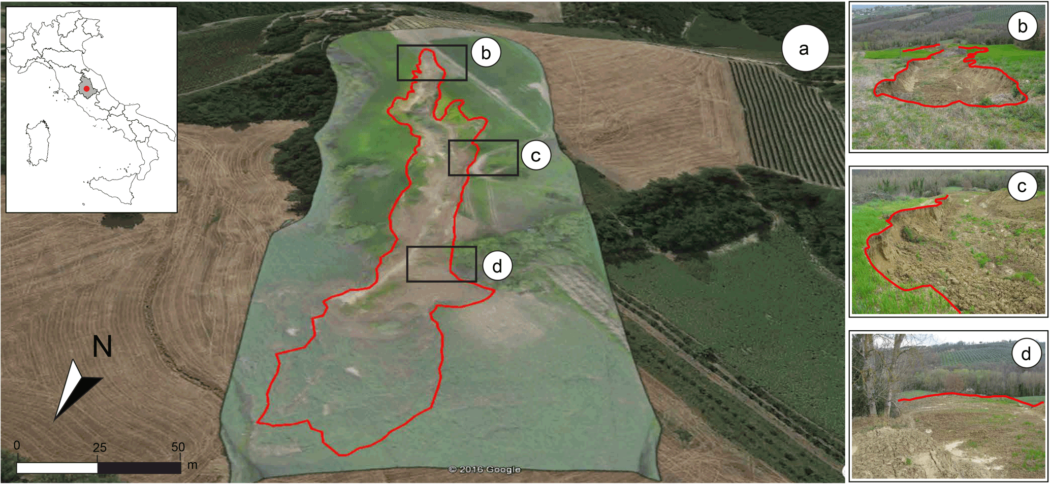
Figure 1 The Assignano landslide, located near Collazzone, Umbria, central Italy. (a) Global view of the landslide. (b) Detail of the landslide source area. (c) Detail of the landslide transportation area. (d) Detail of the landslide deposit. Base image obtained overlaying (“draping”) the image on Google Earth^™. The red line is the boundary of the landslide obtained using the RTK dGPS (benchmark).

Accurate detection of individual landslides has different scopes, including landslide mapping (Di Maio and Vassallo, 2011; Manconi et al., 2014; Plank et al., 2016), landslide hazard analysis and risk assessment (Allasia et al., 2013), to support the installation of landslide monitoring systems (Tarchi et al., 2003; Teza et al., 2007; Monserrat and Crosetto, 2008; Giordan et al., 2013), and for landslide geotechnical characterization and modelling (Gokceoglu et al., 2005; Rosi et al., 2013). Mapping of individual landslides can be executed using the same techniques and tools commonly used by geomorphologists to prepare landslide inventory maps. Such techniques and tools include (a) field survey (Santangelo et al., 2010), (b) heuristic visual interpretation of monoscopic or stereoscopic aerial or satellite images (Brardinoni et al., 2003; Fiorucci et al., 2011; Ardizzone et al., 2013), (c) lidar-derived images (Ardizzone et al., 2007; Van Den Eeckhaut et al., 2007; Haneberg et al., 2009; Giordan et al., 2013; Razak et al., 2013; Niculita et al., 2016, Petschko et al., 2016), (d) ultra-high-resolution images acquired by unmanned aerial vehicles (UAVs; Niethammer et al., 2010; Giordan et al., 2015a, b; Torrero et al., 2015; Turner et al., 2015). Heuristic visual mapping of landslide features is based on the systematic analysis of photographic characteristics such as colour, tone, mottling, texture, shape, and morphological characteristics such as size, curvature, concavity and convexity (Pike, 1988). The mentioned photographic and morphological characteristics encompass all the possible landslide features that can be used for the (visual) image interpretation.

All these mapping techniques have inherent advantages and intrinsic limitations, which depend on the characteristics of the images, including their spatial and spectral resolutions (Fiorucci et al., 2011). The limitations affect differently the mapping, based on the size and type of the investigated landslides. As a result, an image from a single sources or a single mapping technique are “blind” to some landslides features. This inevitably results in an incomplete landslide inventory map. Furthermore, maps can contain errors in terms of the position, size and shape of the mapped landslides (Guzzetti et al., 2000; Galli et al., 2008; Santangelo et al., 2015a).

A few attempts exist to evaluate the errors associated with different types of landslide inventory maps (Carrara et al., 1992; Ardizzone et al., 2002, 2007; Van Den Eeckhaut et al., 2007; Fiorucci et al., 2011; Santangelo et al., 2010; Mondini et al., 2013). Most of them compare maps prepared using aerial or satellite images to maps obtained through reconnaissance field mapping (Ardizzone et al., 2007; Fiorucci et al., 2011) or GPS surveys (Santangelo et al., 2010). Conversely, only a few authors have attempted to evaluate how the characteristics of images acquired from different sources influence landslide detection and mapping (Carrara et al., 1992).

In this work, we evaluate how images of different types and characteristics influence event landslide mapping. We do so by comparing the maps prepared for one rainfall-induced landslide in a pairwise approach, including a benchmark map. The seven maps were obtained using different techniques and images, including (i) a reconnaissance field survey, (ii) the interpretation of ultra-high-resolution images taken by an optical camera on-board of a UAV, and (iii) the visual interpretation of VERY HIGH RESOLUTION (VHR), monoscopic and stereoscopic, multispectral images taken by the WorldView-2 satellite. These comparisons included an eighth map, obtained through dGPS survey, considered as the benchmark showing the “ground truth”. Based on the results of the comparison, we infer the ability of different optical images, with different spectral and spatial characteristics and type (monoscopic or stereoscopic), to portray the landslide features that can be exploited for the visual detection and mapping of landslides. Arguably, the combination of image characteristics, the prevalent landslide signature, the size of the study area and the available resources define the criteria for the optimal selection of remote sensing images for landslide mapping.

2 The Assignano landslide

For our study, we selected the Assignano landslide, a slide earthflow (Hutchinson, 1970) triggered by intense rainfall in December 2013 in the northwest-facing slope of the Assignano village, Umbria, central Italy (Fig. 1). The landslide developed in a crop area, where a layered sequence of sand, silt and clay deposits crop out (Santangelo et al., 2015b). The slope failure is about 340 m long, 40 m wide in the transportation area, and 60 m wide in the deposition area, and is characterized by three distinct source areas, two located on the southwestern side of the landslide and a third located on the northeastern side of the landslide. The source and transportation area has an overall length of about 230 m, and a width increasing from 10 to 40 m from the top of the source area to the bottom of the transportation area. Elevation in the landslide ranges from 276 m along the landslide crown, to 206 m at the lowest tip of the deposit. The source and transportation area is bounded locally by sub-vertical, 2 to 4 m high escarpments. In the landslide, terrain slope averages 11^∘, and is steeper (12^∘) in the source and transportation area than in the deposition area (9^∘). The landslide signature (Pike, 1988) is different in the different parts of the landslide. In the source and transportation area the signature is predominantly photographical (radiometric), whereas in the landslide deposit it is mainly morphological (topographic). The photographic signature consists in all the landslide features that can be detected by the analysis of the photographical characteristics of a given image: colour, tone, pattern and mottling of a given image (Guzzetti et al., 2012). The morphological signature consists in all the landslide features that can be detected by the analysis of the topography – therefore, features such as curvatures, shape, slope, concavity and convexity are always taken into account (Guzzetti et al., 2012). The differences within the landslide allowed us to separate the source and transportation area from the deposition area.

3 Image acquisition

On 14 April 2014, we conducted an aerial survey of the Assignano landslide using an X-shaped frame octocopter with eight motors mounted on four arms (four sets of CW and CCW props) with a payload capacity of around 1 kg, and a flight autonomy of about 20 min. The UAV was equipped with a remotely controlled gimbal hosting a GoPro^® Hero 3 video camera and a Canon EOS M camera. We controlled the flight of the UAV manually, relying on the real-time video stream provided by the GoPro^®. The operational flight altitude of the UAV was kept in the range between 70 and 100 m above the ground. This allowed the Canon EOS M camera to capture 97 digital colour images of the landslide area with a ground resolution of about 2–4 cm, with the single images having an overlap of about 70 % and a side lap of about 40 %. For the accurate geocoding of the images, 13 red-and-white, four-quadrant square targets, 20 cm × 20 cm in size were positioned outside and inside the landslide. The geographical location (latitude, longitude, elevation) of the 13 target centres was obtained using a real-time kinematic (RTK) differential global positioning system (dGPS), with a horizontal error of less than 3 cm. The 97 images were processed using commercial, structure-from-motion software (Agisoft Photoscan^®) to obtain (i) a 3-D point cloud, (ii) a digital surface model (DSM), and (iii) a digital, monoscopic, ultra-high-resolution (ground sampling distance is 3 cm × 3 cm) orthorectified image in the visible spectral range, which we used for the visual mapping of the Assignano landslide (Table 1).

To map the landslide, a stereoscopic pair from the WorldView-2 satellite was used. The satellite stereo pair was taken on 14 April 2014 (the same day of the UAV survey). It has a spatial resolution of 46 cm in panchromatic, and 1.84 m in multispectral, with a 11 bit dynamic range. For the satellite imagery, the rational polynomial coefficients (RPCs) were available, allowing for accurate photogrammetric processing of the images. The RPCs were used to generate 3-D models of the terrain from the stereoscopic image pair. Exploiting the characteristics of the satellite image, four separate images for landslide mapping were prepared, namely (i) a monoscopic, “true colour” (TC) image, (ii) a monoscopic false-colour-composite (FCC) image obtained from the composite near-infrared, red and green (band 4, 3, 2), (iii) a TC stereoscopic pair, and (iv) a FCC stereoscopic pair. A total of four maps of the Assignano landslide were prepared through the visual interpretation of the four images (Table 1). Both satellite and UAV images are free from deep shadows (Fig. 2).

Table 1 Characteristics of the images used to identify and map the Assignano landslide (Fig. 2). O: order in the sequence of images shown to the interpreter. Platform used to capture the image: W, WorldView-2 satellite; U, UAV. Resolution (ground resolution). Spectral (image spectral composite): TCC, true colour composite (red, green, blue); FCC, false-colour composite (near-infrared, red, green). Type (image type): M, monoscopic; S, stereoscopic; P, pseudo-stereoscopic. Map: corresponding landslide map (Fig. 5).

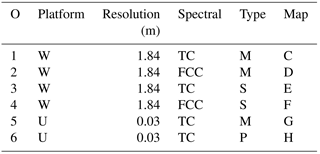
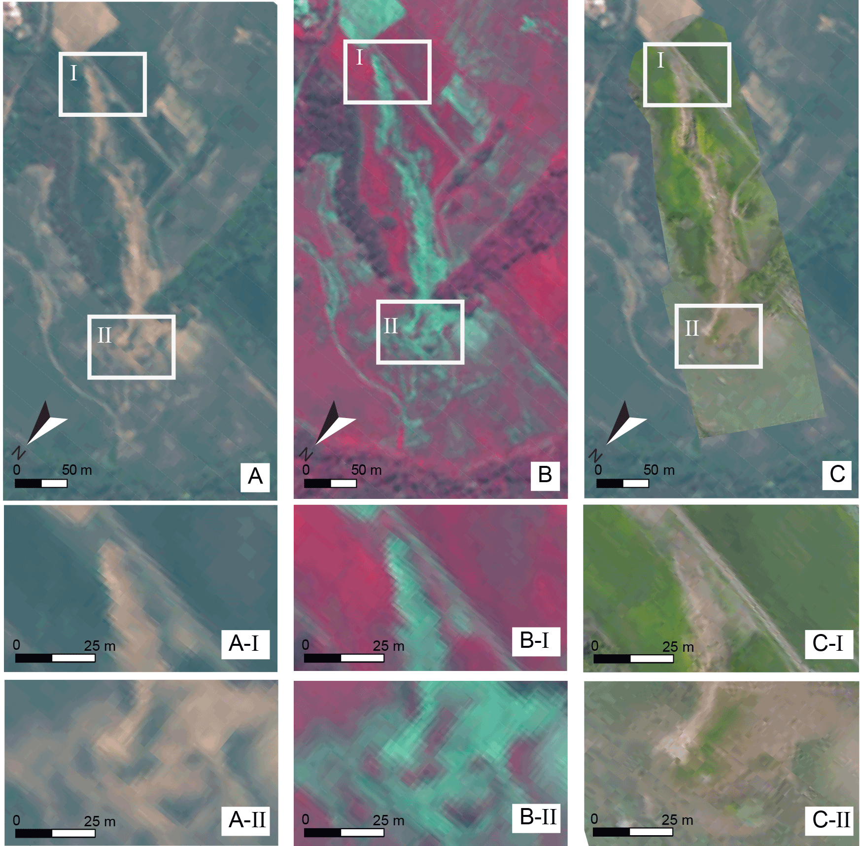
Figure 2 Images used to map the Assignano landslide. (a) TC WorldView-2 satellite image, (aI) detail of the source area and (aII) detail of the landslide deposit. (b) WorldView-2 satellite image in FCC, (bI) detail of the source area and (bII) detail of the landslide deposit. (c) UAV monoscopic image and (cI) a detail of the source area and (cII) a detail of the deposition area.

To compare the images obtained by the UAV and the WorldView-2 satellite, we co-registered the images, and evaluated the co-registration on seven control points (Fig. 3), obtaining a distance root mean square error, DRMS = 0.53 m, and a circular error probability, CEP_50 % = 0.42 m, which was considered adequate for landslide mapping, and for the maps comparison.

4 Landslide mapping

We prepared eight maps of the Assignano landslide using different approaches, images and datasets, including two maps prepared through field surveys, four maps prepared through the visual interpretation of monoscopic and stereoscopic satellite images, and two maps prepared through the visual interpretation of the orthorectified images taken by the UAV (Table 1). The maps are available at https://doi.org/10.17605/OSF.IO/GD2U9.

The field mapping and the image interpretation were carried out by independent geomorphologists. The two geomorphologists who carried out the field activities (the reconnaissance field mapping and the RTK-dGPS survey) were not involved in the visual interpretation of the satellite and the UAV images. Equally, the geomorphologist who interpreted visually the satellite and the UAV images did not take part in the field activities. Visual interpretation of the remotely sensed images was performed by a single geomorphologist to avoid problems related to different interpretation skills by different interpreters (Carrara et al., 1992). The eight maps of the Assignano landslide were then compared adopting a pairwise approach to quantify and evaluate the mapping differences.

Figure 3 Position of the seven GCPs used to evaluate the co-registration of WorldView-2 satellite image (a) and UAV image (b). Corresponding points are illustrated with the same symbol. Differences of the coordinates of the corresponding points along X (E–W direction, ΔX) and along Y (N–S direction, ΔY) are provided in metres on the left of the figure.

The geomorphologist who interpreted visually the images was shown first the 1.84 m resolution, monoscopic satellite image, next the 1.84 m resolution stereoscopic satellite pair, and lastly the 3 cm resolution UAV images. The monoscopic and the stereoscopic satellite images were first shown in TC and then in FCC. Lastly, the interpreter was shown the draped ultra-high-resolution UAV image. Selection of the sequence of the images given to the geomorphologist for the expert-driven visual interpretation was based on the assumption that for landslide mapping (i) the ultra-high-resolution monoscopic images provide more information than the 1.84 m monoscopic or stereoscopic images, (ii) for equal spatial resolution images, stereoscopic images provide more information than monoscopic images, and (iii) for equal image type (monoscopic, stereoscopic), the FCC images provide more information than the TC images. To prevent biases related to possible previous knowledge of the landslide, the interpreter was not shown the results of the reconnaissance field mapping.

4.1 Field mapping

Field mapping of the Assignano landslide consisted in two synergic activities: (i) a reconnaissance field survey, and (ii) a RTK dGPS aided survey. First, the reconnaissance field survey was conducted by two geomorphologists (FF and MR) who observed the landslide and took photographs of the slope failure from multiple viewpoints, close to and far from the landslide. The geomorphologists drew in the field a preliminary map of the landslide exploiting the most recent satellite image available at the time in Google Earth^™, which was a pre-event image taken on 8 July 2013 (Fig. 4). The reconnaissance field mapping was then refined in the laboratory using the ground photographs taken in the field. We refer to this reconnaissance representation of the Assignano landslide as “Map B”.

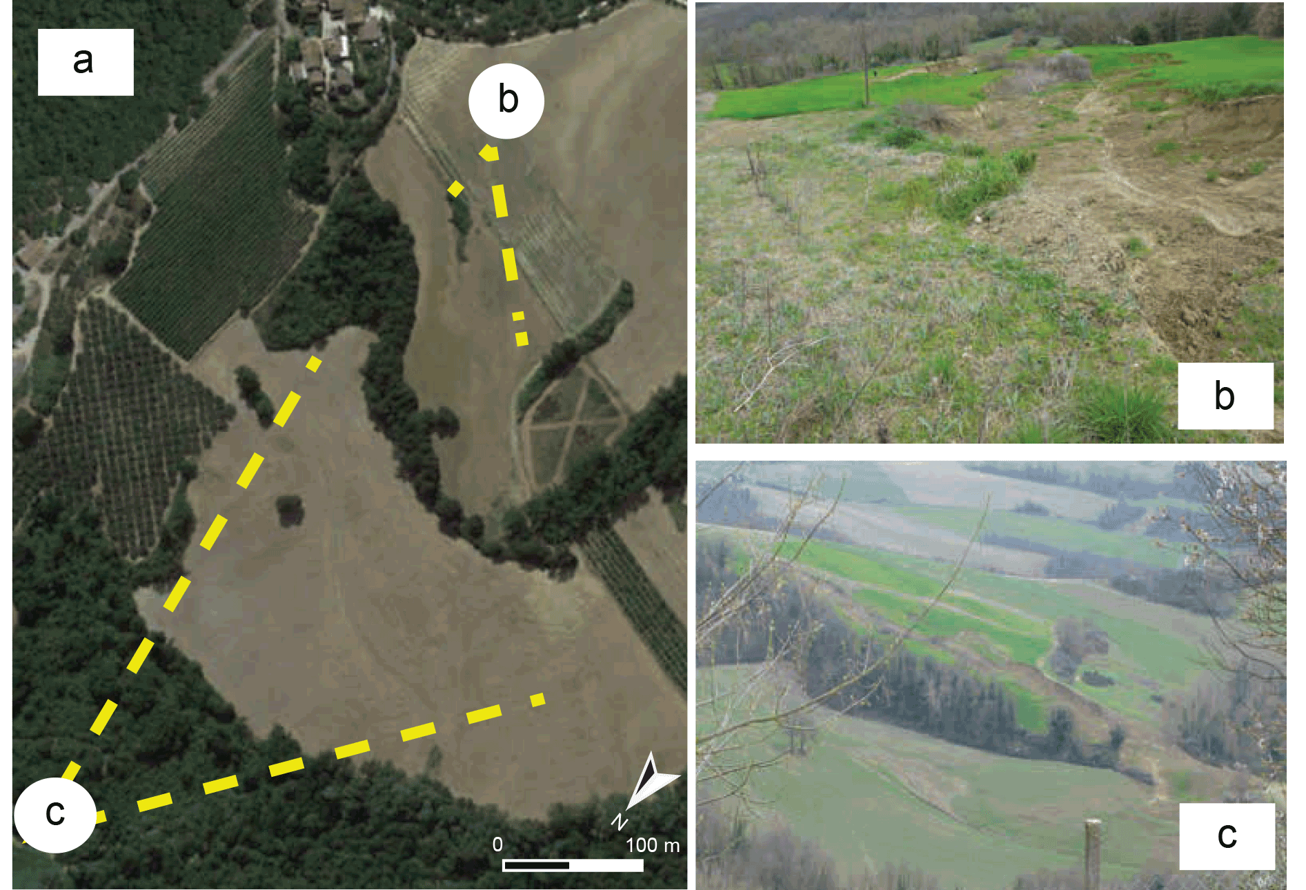
Figure 4 (a) Overview of the Assignano landslide area in Google Earth^™ taken on 8 July 2013. Photo shooting points and photograph taken (b) close to the landslide and (c) from a viewpoint. The photographs taken in the field and the Google Earth^™ image were used to prepare the reconnaissance field map.

Next, the same two geomorphologists (FF and MR) conducted an RTK dGPS-aided survey walking a Leica Geosystems GPS 1200 receiver along the landslide boundary, capturing 3-D geographic coordinates every about 5 m, in 3-D distance. For the purpose, the SmartNet ItalPoS real-time network service was used to transmit the correction signal from the GPS base station to the GPS roving station. The estimated accuracy obtained for each survey point measured along the landslide boundary was 2 to 5 cm, measured by the root mean square error (RMSE), on the ETRF-2000 reference system. The cartographic representation of the Assignano landslide produced by the RTK dGPS survey is referred to as “Map A”, and is considered as the benchmark against which to compare the other maps. Mapping a landslide by walking a GPS receiver around its boundary is an error-prone operation – e.g. because in places the landslide boundary is not sharp, or clearly visible from the ground (Santangelo et al., 2010). Nevertheless, this is the most reasonable working assumption (Santangelo et al., 2010). Furthermore, the geometrical information obtained by walking a GPS receiver along the landslide boundary was superior to the information obtained through the reconnaissance field mapping (Map B).

4.2 Mapping through image interpretation

A trained geomorphologist (MS) used the three monoscopic images (the TC and FCC monoscopic satellite images, and the monoscopic ultra-high-resolution UAV image) to perform a heuristic, visual mapping of the Assignano landslide. For this purpose, the interpreter considered the photographic (colour, tone, mottling, texture) and geometric (shape, size, pattern of individual terrain features, or sets of features) characteristics of the images (Antonini et al., 2002). In this way, the geomorphologist prepared (i) “Map C” interpreting visually the monoscopic TC satellite image, (ii) “Map D” interpreting visually the monoscopic FCC satellite image, and (iii) “Map G” interpreting visually the monoscopic TC UAV image (Table 1).

Next, the interpreter used the two stereoscopic satellite images (the TC and FCC images) to prepare “Map E” and “Map F” (Table 1). In the stereoscopic images, the photographic and morphological information is combined, favouring the recognition of the landslide features through the joint analysis of photographic (colour, tone, mottling, texture), geometrical (shape, size, pattern of features), and morphological terrain features (curvature, convexity, concavity). To analyse visually the stereoscopic satellite images, the interpreter used the StereoMirror^™ hardware technology, combined with the ERDAS IMAGINE^® and Leica Photogrammetry Suite (LPS) software. To map the landslide features in real-world, 3-D geographical coordinates, the interpreter used a 3-D floating cursor (Fiorucci et al., 2015).

To interpret visually the ultra-high-resolution UAV image, the interpreter overlaid (“draped”) the image on Google Earth^™. For the purpose, we first treated the UAV image with the gdal2tiles.py software to obtain a set of image tiles compatible with Google Earth^™ terrain visualization platform. To the best of our knowledge, the platform is the only free 2.5-D image visualization environment that allows the editing of vector (point, line, polygon) information. Other commercial (e.g. ArcScene) and open source (e.g. ParaView, GRASS GIS), 2.5-D visualization tools do not provide editing capabilities. Google Earth^™ is a user-friendly solution for mapping single landslides, and for preparing landslide event inventories for limited areas, with the possibility for the user to visualize a landscape from virtually any viewpoint, facilitating landslide mapping. The representation of the landslide obtained through the visual interpretation of the ultra-high-resolution UAV image is referred to as “Map H”.

For the visual interpretation of the satellite and the UAV images, the interpreter adopted a visualization scale in the range from 1:1000 to 1:6000, depending on the image spatial resolution (Table 1). The scale of observation was selected to obtain the best readability of each landslide feature and the surroundings. Despite the fact that the maps were produced at slightly different observation scales, the differences arising from the comparison are due to actual features (e.g. the image resolution and radiometry), and not to the different observation scales.

5 Results

Using the described mapping methods, and the available satellite and UAV images (Table 1), we prepared eight separate and independent cartographic representations of the Assignano landslide, shown in Fig. 5 as Map A to Map H.

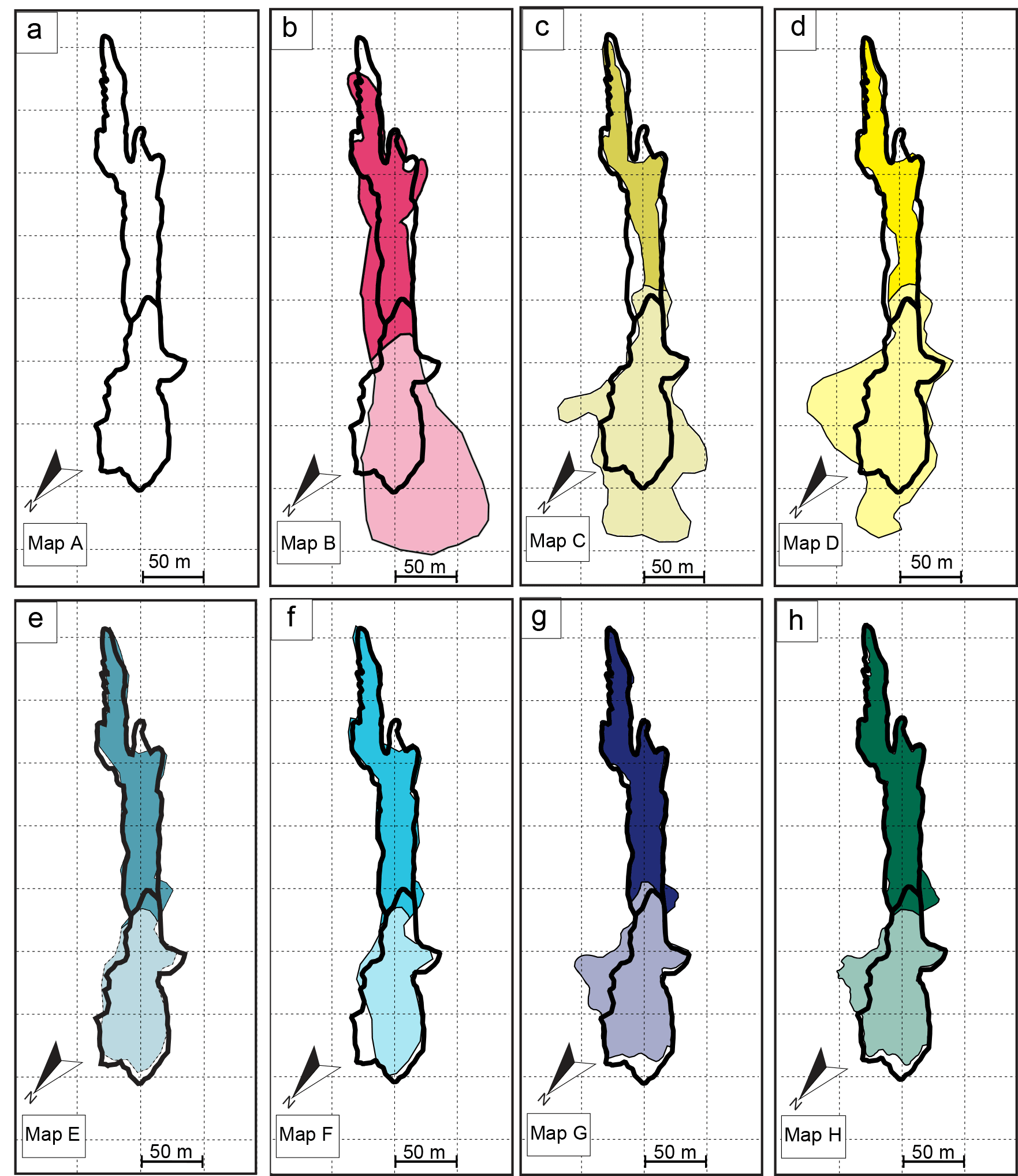
Figure 5 Eight independent cartographic representations of the Assignano landslide, “Map A” to “Map H”. Map A, obtained through a RTK dGPS survey, is considered the “benchmark”, and is shown as a thick black line in the other maps. Map B is obtained through reconnaissance field mapping. Maps C–F are obtained through the expert visual interpretation of the satellite images. Maps G and H are obtained through the expert visual interpretation of the orthorectified image taken by the UAV. See Table 1 for image characteristics. Dark colours show the landslide source and transportation area. Visual inspection of the images reveals the maps most similar to the benchmark.

Considering the entire landslide, visual inspection of Fig. 5 reveals that the map most similar to the benchmark (Map A) is Map E, prepared examining the TC stereoscopic satellite image. Conversely, the largest differences were observed for the landslide maps obtained through the reconnaissance field survey (Map B), and the visual interpretation of the monoscopic satellite images (Map C and Map D). Considering only the source and transportation areas (dark colours in Fig. 5), interpretation of the UAV ultra-high-resolution images resulted in the landslide maps most similar (Map G and Map H) to the benchmark (Map A). It is worth noting the systematic lack in the mapping of one of the two secondary landslide source areas located in the SW side of the landslide, which was recognized only from the visual inspection of the ultra-high-resolution orthorectified images taken by the UAV. In the field, this secondary source area was characterized by small cracks along the escarpment and a limited disruption of the meadow, making it particularly difficult to be detected and mapped. We argue that only the ultra-high-resolution images allowed for the detection of the cracks. Considering only the landslide deposit (light colours in Fig. 5), the landslide mapping that was more similar to the benchmark (Map A) was obtained interpreting the TC, stereoscopic satellite images (Map E). We also note that in most of the maps the landslide deposit was mapped larger (Map G, Map H) or much larger (Map B, Map C and Map D) than the benchmark (Map A).

Table 2 Comparison of the total landslide area (A_L), the landslide source and transportation area (A_LS), the landslide deposit (A_LD), the width and length of the entire landslide (W_L, L_L), of the source and transportation area (W_LS, L_LS), and of the deposit (W_LD, L_LD), for eight separate and independent cartographic representations of the Assignano landslide. EL, entire landslide; ST, landslide source and transport area; LD, landslide deposit. See Table 3 for the characteristics of the single maps.

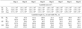
Table 2 lists geometric measures of the mapped landslides, including the planimetric measurement of length, width and area (i) of the entire landslide, (ii) of the landslide source and transportation area (dark colours in Fig. 5), and (iii) of the landslide deposit (light colours in Fig. 5). The length and width measurements were obtained in a GIS as the length and the width of the minimum oriented rectangle encompassing (i) the entire landslide, (ii) the landslide source and transportation area, and (iii) the landslide deposit. Our benchmark (Map A) has a total area A_L = 1.1 × 10⁴ m², and is L_LS = 362 m long and W_LS = 71 m wide. Amongst the other seven maps (Map B to Map H in Fig. 5), the largest landslide is shown in Map B, obtained through the reconnaissance field mapping, and has A_L = 1.91 × 10⁴ m², 71.1 % larger than the benchmark. Conversely, the smallest landslide is shown in Map F, with A_L = 1.1 × 10⁴ m², 4.6 % smaller than the benchmark. The longest and largest landslide is found in Map C, with L_LS = 405 m (11 % longer than the benchmark) and W_LS = 113 m (60 % wider than the benchmark).

Considering the source and transportation area, in Map A (the benchmark) A_LS = 5.4 × 10³ m², L_LS = 228 m and W_LS = 52 m. The largest representation of the source and transportation area is found in Map B (reconnaissance field mapping) with A_LS = 7.4 × 10³ m², 36.9 % larger than the benchmark, and the smallest source and transportation area is found in Map G, with A_LS = 5.2 × 10³ m², 3.6 % smaller than the benchmark. The longest source and transportation area is found in Map F, with L_LS = 239 m, 5 % longer than the benchmark, and the shortest source and transportation area is shown in Map C, with L_LS = 206 m, 9.7 % shorter than the benchmark. The largest source and transportation area is shown in Map B, W_LS = 60 m, 15.7 % wider than Map A, and the narrowest source and transportation area is in Map C, L_LS = 44 m, 15.3 % narrower than the benchmark. Considering instead only the landslide deposit, our benchmark (Map A) has A_LD = 5.7 × 10³ m², L_LS = 153 m and W_LS = 61 m. The largest deposit is shown in Map B (reconnaissance field mapping) and has A_LD = 1.2 × 10⁴ m², 103.4 % larger than the benchmark, whereas the smallest landslide deposit is shown in Map F, with A_LD = 4.6 × 10³ m², 19.8 % smaller than the benchmark. Analysis of the length and width of the landslide deposit reveals that Map C shows the longest deposit, L_LS = 206 m, 35 % longer than the benchmark, and Map H shows the shortest deposit, L_LS = 122 m, 20.2 % shorter than the benchmark. Similarly, the largest landslide deposit is shown in Map C, W_LS = 112 m, 82.8 % wider than the benchmark, and the narrowest landslide deposit is portrayed in Map E, W_LS = 56 m, 8.2 % less than the benchmark.

To compare quantitatively the different landslide maps, we use the error index E proposed by Carrara et al. (1992), adopting the pairwise comparison approach proposed by Santangelo et al. (2015a). The index provides an estimate of the discrepancy (or similarity) between corresponding polygons in two maps, and is defined as

$$\begin{array}{}\text{(1)}& {\displaystyle }E={\displaystyle \frac{\left(A\cup B\right)-\left(A\cap B\right)}{\left(A\cup B\right)}};\mathrm{0}\le E\le \mathrm{1},\end{array}$$

where A and B are the areas of two corresponding polygons in the compared maps, and ∪ and ∩ are the geographical (geometric) union and intersection of the two polygons, respectively. E spans the range from 0 (perfect matching) to 1 (complete mismatch).

We compared the eight maps of the Assignano landslide (Fig. 5) adopting a pairwise approach, and considering first only the landslide source and transportation area, next only the landslide deposit, and lastly the entire landslide. Figure 6 summarizes the 84 values of the error index E: 28 for the landslide source and transportation area (Fig. 6I), 28 for the landslide deposit (Fig. 6II) and 28 for the entire landslide (Fig. 6III). On average, the source and transportation area exhibits values of the error index smaller than the values found in the landslide deposit. This indicates that in the source and transportation area the landslide maps are more similar than in the landslide deposit. Inspection of Fig. 6I reveals a decrease of the error index in the source and transportation area for the maps obtained interpreting the available images (from Map C to Map H), compared to our benchmark obtained through the RTK dGPS survey (0.15 $\le E\le$ 0.38), with Map G obtained interpreting the TC, monoscopic, ultra-high-resolution UAV image. In the landslide deposit (Fig. 6II), the minimum difference (E = 0.21) was found comparing the benchmark to Map E, obtained through the interpretation of the stereoscopic TC satellite image, and the largest difference (E = 0.52) was found comparing the benchmark to Map C, prepared interpreting the TC, monoscopic, satellite image.

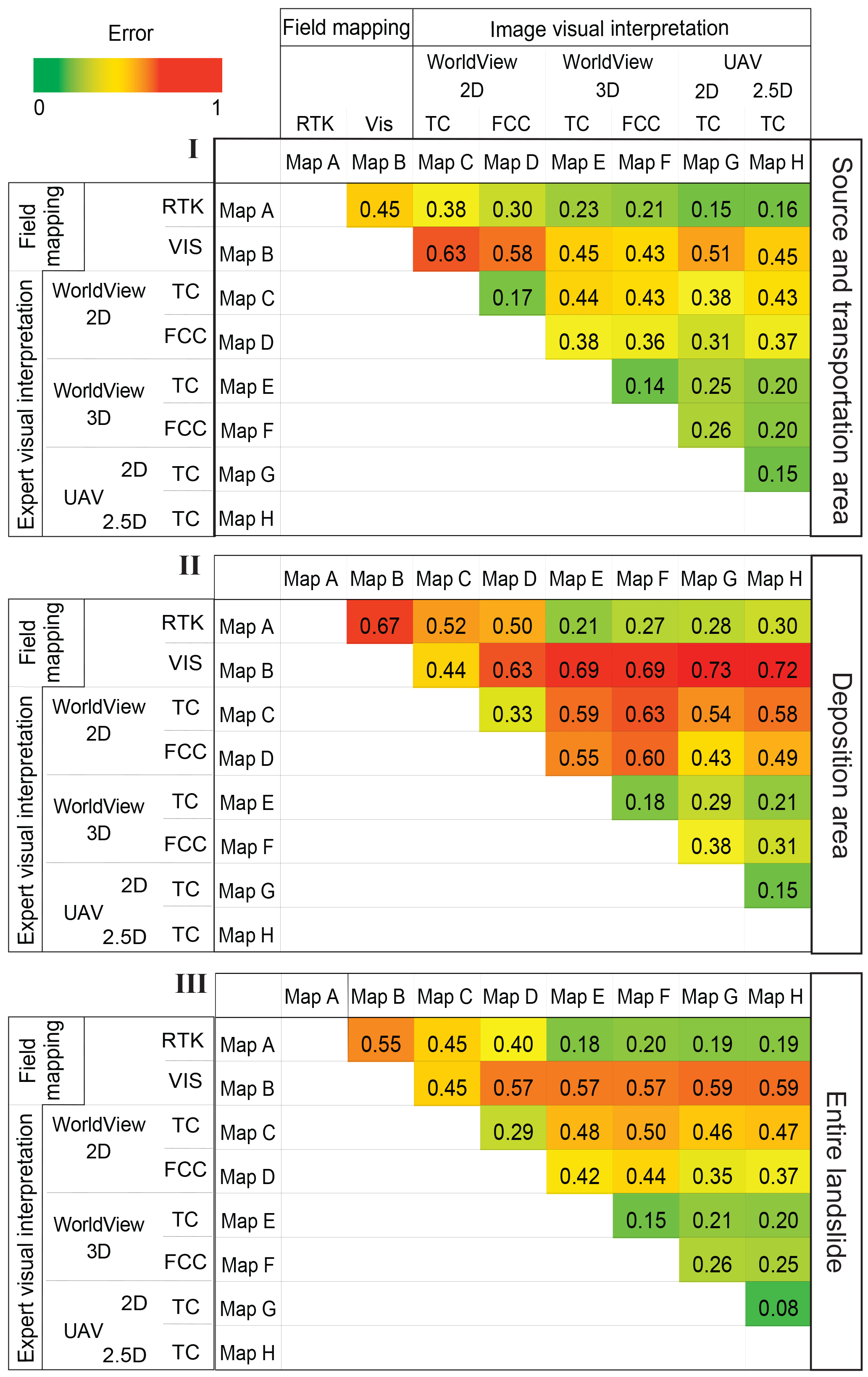
Figure 6 The error index (E) proposed by Carrara et al. (992), was used to compare quantitatively the different landslide maps. (I) Error index matrix for the landslide source and transportation area. (II) Error index matrix for the landslide deposit. (III) Error matrix for the entire landslide. E spans the range from 0 (perfect matching) to 1 (complete mismatch).

Comparison of the maps obtained through the interpretation of the monoscopic images (Map C and Map D), and the maps obtained through the interpretation of stereoscopic (Map E and Map F) or ultra-high-resolution images (Map G and Map H), reveals high values of the error index, which is slightly worse in the landslide deposit. This is evident in the source and transportation area (0.31 ≤ E ≤ 0.44; Fig. 6I), and in the landslide deposit (0.43 ≤ E ≤ 0.63; Fig. 6II). Map C and Map D are very similar, with a mapping error E = 0.17. Maps obtained through the interpretation of stereoscopic satellite images (Map E and Map F, prepared using TC and FCC images, respectively), and maps prepared by interpreting the UAV images (Map G and Map H), exhibit a generally low value of E. In particular, 0.14 ≤ E ≤ 0.26 in the landslide source and transportation area, and 0.15 ≤ E ≤ 0.38 in the landslide deposit. The reconnaissance field mapping (Map B) exhibited the largest differences compared to all the other maps (0.63 ≤ E ≤ 0.45) in the landslide source and transportation area, and 0.44 ≤ E ≤ 0.73 in the landslide deposit. The large values of E in the landslide deposit is probably due to lack of visibility of part of the landslide toe in the field.

6 Discussion

In this section, the ability of the different images to resolve the landslide photographical and morphological signatures is discussed, considering separately (i) the image spatial and (ii) spectral resolutions, and (iii) the image type (monoscopic, stereoscopic, or pseudo-stereoscopic). Each of these three factors is considered separately, keeping the other two factors constant.

Inspection of Fig. 6I reveals that the maps of the landslide source and transportation area obtained from images characterized by the highest spatial resolution (Map G and Map H) exhibit the smallest errors when compared to the benchmark. The mapping error obtained for Map C (TC, monoscopic) is 2.5 times larger than the error obtained using the ultra-high-resolution orthorectified images taken by the UAV, whereas the error obtained from Map E (TC, stereoscopic) is smaller, and about 1.5 times larger than the error obtained for Map H (TC, pseudo-stereoscopic). In the landslide deposit (Fig. 6II), the map obtained exploiting the monoscopic, TC satellite image exhibits an error 1.7 times larger than the error obtained using Map G (TC, monoscopic UAV). Conversely, the error is smaller in the map obtained from the 2 m spatial resolution, stereoscopic TC satellite image (Map E) than from the 3 cm spatial resolution, pseudo-stereoscopic image taken by the UAV (Map H). Collectively, the pairwise comparisons highlight an improvement of the quality of the mapping of the landslide features that exhibits a distinct photographical signature, most visible in the source and transportation area of the Assignano landslide, with an increase of the image spatial resolution (Fig. 6). Use of the ultra-high-resolution image captured by the UAV did not result in an improvement of the mapping in the deposition area of the Assignano landslide, where the landslide exhibits a distinct morphological signature. Furthermore, most of the landslide parts that were not identified in the maps prepared using the satellite image are covered by vegetation, locally bounded by small and thin cracks with an average width smaller than the size of the 2 × 2 m pixel. In the satellite image, the cracks are located in pixels containing a mix of vegetation and bare soil, making it difficult for the interpreter to recognize the cracks.

Next, we evaluate the effectiveness of the image spectral resolution, and for the purpose we examine the mapping errors of Maps C and Map E (TC), and of Map D and Map F (FCC). The mapping of the source and transportation area prepared using the FCC images (Map D and Map F) resulted in smaller errors than the mapping prepared using the corresponding TC images (Map C and Map E), for both monoscopic and stereoscopic images (Fig. 6I). In the source and transportation area, the FCC emphasized the presence or absence of the vegetation, and contributed locally to highlight the typical photographical signature of the landslide. Conversely, in the landslide deposition area (Fig. 6II) use of the FCC images did not result in a systematic reduction of the mapping error, when compared to the TC images. We conclude that use of the additional information contributed by the near-infrared (NIR) band in the 1.84 m resolution satellite image did not improve the quality of the mapping. On the other hand, the contribution of the NIR in the 3 cm UAV image remains unknown.

Lastly, the influence of the image type (monoscopic, stereoscopic, pseudo-stereoscopic) on the mapping error was evaluated by comparing (i) the TC images (Map C and Map E), (ii) the FCC images (Map D and Map F), and (iii) the ultra-high-resolution UAV image (Map G and Map H). Comparison of the TC, monoscopic (Map C) and stereoscopic (Map E) images revealed a mapping error for the entire landslide, with the mismatch larger in the deposition area than in the source and transportation area (Fig. 6). A similar result was obtained comparing the FCC, monoscopic (Map D) and stereoscopic (Map F) images with a mapping error for the entire landslide, and again the mismatch is larger in the deposition area (E= 0.60) than in the source and transpiration area (E= 0.36). In the deposition area, where the morphological signature of the Assignano landslide is strongest, the mapping error obtained comparing the benchmark (Map A) to the landslide maps prepared using the monoscopic images (Map C and Map D) is 2 times larger than the error observed for the maps prepared using the corresponding stereoscopic images (Map E and Map F). The differences are smaller in the source and transportation area, where the morphological signature of the landslide is less distinct. Comparison of Map E (TC, stereoscopic) and Map F (FCC, stereoscopic) for the entire landslide reveals a very small mapping error, indicating the similarity of the two maps, which were also very similar to the benchmark (Map A).

Comparison for the entire landslide of the maps prepared using the ultra-high-resolution images captured by the UAV (Map G and Map H) exhibits the smallest error of all the pairwise comparisons (Fig. 6III), indicating the large degree of matching between the two maps. The degree of matching is only marginally smaller in the source and transportation area, and in the deposition area. When compared to the benchmark (Map A), Map G and Map H exhibit a small error for the entire landslide, which is larger in the deposition area and slightly smaller in the source and transportation area. Interestingly, the mismatch with Map A (the benchmark) is lower for the monoscopic (Map G) than for the pseudo-stereoscopic (Map H) map. The finding highlights the lack of an advantage in using a pseudo-stereoscopic (2.5-D) image for mapping the landslide. We attribute this result to the low resolution of the (pre-event) digital elevation model (DEM) used to drape the ultra-high-resolution image for visualization purposes, which did not add any significant morphological information to the expert visual interpretation.

Table 3 Comparison of the estimated cost, acquisition and pre-processing time, and storage requirement for an area of 4 km² (2 km × 2 km) and for an area of 100 km² (10 km × 10 km), for monoscopic and stereoscopic satellite images, and for an area of 15 km² for photographic images captured by a UAV.

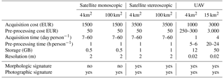
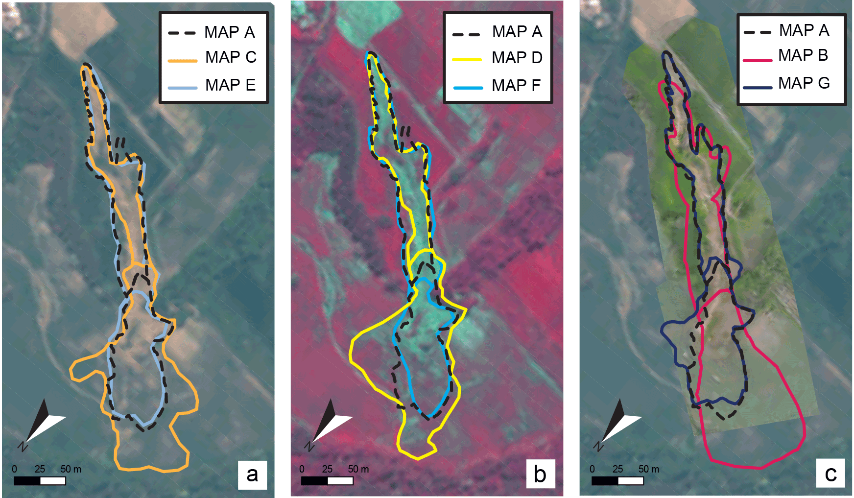
Figure 7 Comparison of landslide maps prepared for the Assignano landslide, Umbria, central Italy. (a) Landslide map obtained from a monoscopic (Map C, dark yellow line) and a stereoscopic (Map E, light blue line), true-colour (TC) WorldView-2 satellite image (base image), and a mapping of the landslide obtained by walking a GPS receiver along the landslide boundary (Map A, black line). (b) Landslide map obtained from a monoscopic (Map D, yellow line) and a stereoscopic (Map F, cyan line), false-colour-composite (FCC) WorldView-2 satellite image, and a mapping obtained by walking a GPS receiver along the landslide boundary (Map A, black line). (c) Landslide map obtained from field survey (Map B, pink line) and from a monoscopic, TC, ultra-high-resolution image captured by a UAV (Map G, purple line), and the mapping obtained by walking a GPS receiver along the landslide boundary (Map A, black line).

Joint analysis of Figs. 5b and 6 reveals that, when compared to the benchmark (Map A), the reconnaissance field mapping (Map B) exhibited the largest mapping error of all the performed pairwise comparisons, with E= 0.45 in the source and transportation area, E= 0.67 in the landslide deposit, and E= 0.55 for the entire landslide. Our results are similar to the results of tests performed to compare field-based landslide maps against GPS-based surveys of single landslides (Santangelo et al., 2010), the visual interpretation of very-high resolution stereoscopic satellite images (Ardizzone et al., 2013), or the semi-automatic processing of monoscopic satellite images (Mondini et al., 2013), and confirm the inherent difficulty in preparing accurate landslide maps in the field, unless the mapping is supported by a GPS survey or a similar technology.

The experiment showed that the mapping of the Assignano landslide obtained exploiting the ultra-high-resolution images captured by the UAV (Map G and Map H) was comparable to the maps obtained using the high-resolution stereoscopic satellite image (Map E and Map F), and to the ground-based RTK dGPS survey (Map A, the benchmark). The ultra-high-resolution images and the stereoscopic satellite images are well suited to map event landslides, at least in physiographical settings similar to the one of this study area, and for landslides similar to the Assignano landslide (slide earthflow). For event landslide mapping, selection between ultra-high-resolution pseudo-stereoscopic UAV images and very-high resolution stereoscopic satellite images depends on (i) the extent of the investigated area, (ii) the available resources, including time and budget, and (iii) the accessibility to the study area. The selection is largely independent of the landslide signature, at least for landslides similar to the Assignano landslide. From an operational perspective, modern multi-rotor UAVs allow for the acquisition of ultra-high-resolution images over small areas in a limited time, and at very low costs. UAV-based surveys are flexible in their acquisition planning, and partly independent from the local lighting conditions, including the cloud cover. As a drawback, UAVs are strongly (and negatively) affected by wind speed and weather conditions, they allow for a limited flight time (currently approximately 20 min in optimal conditions), which is reduced in bad weather conditions and in cold environments, and typically have limited data storage capacity. Further, it must be possible for the pilot to be at the same time near to the area to be surveyed and to maintain a safe distance from the UAV, a condition that may be difficult to attain in remote or in mountain areas. Collectively, the intrinsic advantages and limitations of modern UAVs make the technology potentially well suited for the acquisition of ultra-high-resolution images for event, seasonal, and multi-temporal mapping of single landslides, of multiple landslides in a single slope, or in a relatively small area (a few hectares). The use of UAV images was recently proposed by Turner et al. (2015) for determining landslide dynamics, exploiting time series of images that can be constructed using UAVs. The result is achievable thanks to centimetre co-registration accuracy of the UAV images. Use of UAVs becomes impracticable with the increasing extent of the study area, largely due to (i) the operational difficulty of flying UAVs over large areas (more than a few square kilometres), and (ii) the acquisition and image processing time and associated cost, which increase rapidly with the size of the study area (Table 3). On the other hand, very high resolution, stereoscopic satellite images also have advantages and limitations for the production of event, seasonal and multi-temporal landslide inventory maps (Guzzetti et al., 2012). The main advantage of the satellite images is that they cover large or very large areas (tens to hundreds of square kilometres) in a single frame with a sub-metre resolution well suited for landslide mapping through the expert visual interpretation of the images (Ardizzone et al., 2013). On the other hand, limitations remain due to distortions caused by different off-nadir angles in successive scenes, and to difficulties – in places severe – of obtaining suitable (e.g. cloud-free) images at the required time intervals. This is particularly problematic for the production of seasonal and multi-temporal landslide maps. Information on the photographic or morphological signature of the typical, or most abundant, landslides in an area, is important to selecting the optimal characteristics of the images best suited for the production of an event, seasonal or multi-temporal landslide inventory map. Use of images of non-optimal characteristics for a typical landslide signature in an area may condition the quality (completeness, positional and thematic accuracy) of the landslide inventory. Where possible, we recommend that the acquisition of images used for the production of event, seasonal or multi-temporal landslide inventory maps is planned considering the typical landslide signature, in addition to the purpose (event inventory, planning of monitoring systems), scale of the mapping (regional or slope scale), and the size and complexity of the study area (Table 3).

7 Concluding remarks

The experiment aimed at determining and measuring the effects of the image characteristics on event landslide mapping. The study was conducted on a slide earthflow (Fig. 1) triggered by intense rainfall in December 2013 in the northwest-facing slope of the Assignano village, Umbria, central Italy. The landslide exhibited a predominant photographical (radiometric) signature in the source and transport area, and a more distinct morphological (topographic) signature in the deposition area.

Increasing the spatial resolution allows us to reduce the error of landslide mapping where landslides show mainly a photographical signature. Such a behaviour was observed in the landslide source and transport area. Here, the image photographic (radiometric) characteristics (true-colour, false-colour composite) and the image type (monoscopic, stereoscopic) played a minor role in augmenting the quality of the landslide maps. Conversely, in the deposition area, where the signature of the landslide was primarily morphological (topographical), mapping errors decreased using stereoscopic satellite images that allowed us to detect topographic features distinctive of the landslide.

FCC and TC in the stereoscopic satellite images give similar values of the error. This indicates that the spectral resolution of the images does not provide useful information to recognize and map the landslide morphological features. On the other hand, the high spatial resolution provided by the UAV images reduces the error, when compared to the monoscopic satellite imagery. However, the error obtained using the UAV images remains higher than that obtained using stereoscopic satellite images, despite the latter having a pixel 1 order of magnitude larger than the UAV images. We conclude that the increase in the spatial resolution improves the ability to map morphological features when using monoscopic images.

Use of the stereoscopic satellite images resulted in more accurate landslide maps (lower error index E) than the corresponding monoscopic images in the landslide deposition area, where the signature of the landslide was primarily morphological. This was expected, as the stereoscopic vision allowed us to better capture the 3-D terrain features typical of a landslide (Pike, 1988), including curvature, convexity and concavity. Conversely, visual examination of the FCC images resulted in more accurate maps than the corresponding TC images in the landslide source and transport area, where the signature of the landslide was primarily photographic. Expert visual interpretation of pseudo-stereoscopic ultra-high-resolution images failed to provide better results than the corresponding monoscopic ultra-high-resolution images, most probably because the DEM used to drape (overlay) the image on the terrain information was of low resolution.

The ultra-high-resolution (3 cm × 3 cm) image captured by the UAV proved to be very effective to detect and map the landslide. The expert visual interpretation of the monoscopic ultra-high-resolution image provided mapping results comparable to those obtained using the about 2 m resolution stereoscopic satellite image.

A comparative analysis of the technological constraints and the costs of acquisition and processing of ultra-high-resolution imagery taken by UAV, and of high, or very high resolution imagery taken by optical satellites, revealed that the ultra-high-resolution images are well suited to map single-event landslides, clusters of landslides in a single slope, or a few landslides in nearby slopes in a small area (up to a few square kilometres; Giordan et al., 2017), and proved unsuited to cover large and very large areas, where the stereoscopic satellite images provide the most effective option (Boccardo et al., 2015).

The field-based reconnaissance mapping (Map B) provided the least accurate mapping results, measured by the largest mapping error when compared to the benchmark map. Results confirm the inherent difficulty in preparing accurate landslide maps in the field through a reconnaissance mapping (Santangelo et al., 2010).

Although the study was conducted on a single landslide (Fig. 1), the findings are general, and can be useful to decide on the optimal imagery and technique to be used when planning the production of a landslide inventory map. The technique and imagery used to prepare landslide inventory maps should be selected depending on multiple factors, including (i) the typical or predominant landslide signature (photographic or morphological), (ii) the scale and size of the study area (a single slope, a small catchment, a large region), and (iii) the scope of the mapping (event, seasonal, multi-temporal; Guzzetti et al., 2012).