Potential impact of climate change and extreme events on slope land hazard – a case study of Xindian watershed in Taiwan

The production and transportation of sediment in mountainous areas caused by extreme rainfall events that are triggered by climate change is a challenging problem, especially in watersheds. To investigate this issue, the present study adopted the scenario approach coupled with simulations using various models. Upon careful model selection, the simulation of projected rainfall, landslide, debris flow, and loss assessment was integrated by connecting the models' input and output. The Xindian watershed upstream from Taipei, Taiwan, was identified and two extreme rainfall scenarios from the late 20th and 21st centuries were selected to compare the effects of climate change. Using sequence simulations, the chain reaction and compounded disaster were analysed. Moreover, the potential effects of slope land hazards were compared for the present and future, and the likely impacts in the selected watershed areas were discussed with respect to extreme climate. The results established that the unstable sediment volume would increase by 28.81 % in terms of the projected extreme event. The total economic losses caused by the chain impacts of slope land disasters under climate change would be increased to USD 358.25 million. Owing to the geographical environment of the Taipei metropolitan area, the indirect losses of a water supply shortage caused by slope land disasters would be more serious than direct losses. In particular, avenues to ensure the availability of the water supply will be the most critical disaster prevention topic in the event of a future slope land disaster. The results obtained from this study are expected to be beneficial because they provide critical information for devising long-term strategies to combat the impacts of slope land disasters.

1 Introduction

In recent years, the frequency and magnitude of disasters associated with extreme climatological events have increased (IPCC, 2012). Studies have established that under extreme climatic conditions, changes in temperature and precipitation can lead to slope land hazards such as landslides and debris flow in the local area (Hsu et al., 2011). For instance, the increasing landslide activity triggered by human-induced climate change has been examined and proved using a projected climate scenario approach at several sites (Buma and Dehn, 1998; Collison et al., 2000; Crozier, 2010). Due to the increasing frequency of extreme precipitation events, the frequency and magnitude of debris flow events also found an increasing trend by a past data set (Rebetez et al., 1997; Stoffel et al., 2014). However, in slope land problems, the various types of hazard are strongly linked or occur as a chain reaction. For example, landslide mass is one of the triggering factors of debris flow. The discussion on the meteorological properties of climate change and one of the consequent hazards, such as rainfall-triggered landslides or rainfall-triggered debris flow, is not enough to describe the impact on slope land.

In slope land hazards, sediment production and transport warrant a great deal of attention. The sequence of events from sediment production to its transport can be regarded as a chain reaction in the watershed. For example, in Taiwan, heavy rainfall triggered by typhoons usually leads to large-scale landslides on slope land. When loose landslide deposits mix with the run-off or dammed lake water, the debris flows downstream along the gully. Hence, the chain reaction of sediment flow cannot be ignored and should be considered in the sediment-related discussions of mountainous terrains, especially in an extreme rainfall event. In this process, the various physical mechanisms could be simulated by an effective combination of models, such as rainfall, landslide, and debris flow.

Furthermore, slope land disasters result in serious casualties and economic loss. For example, Taipei experienced heavy rainfall during Typhoon Soudelor in August 2015. The accumulated rainfall over a period of 3, 6, 12, and 72 h in Xindian watershed (Fushan meteorological station) exceeded 253, 442, 655, and 792 mm, respectively (Wei et al., 2015). Large-scale landslides and debris flows were triggered within this short period because of the intense rainfall. The regional landslide disasters necessitated the closure of roads and the debris flow from the tributaries increased the concentration of suspended solids in the Nanshi River. According to the Taipei Water Department, the peak turbidity reached 39 300 NTU (nephelometric turbidity unit) at 08:00 h on 8 August 2015, and it took 42 h for the value to fall to the permissible limit of 3000 NTU. Because of the disaster, water supply was disrupted and the water quality was compromised on the subsequent days in the Taipei area. Therefore, loss assessment should be used to evaluate the economic impacts of slope land disasters. Both direct losses on slope land and indirect losses downstream of the city must be included, especially with the increasing threat of typhoon events.

In the present study, the scenario approach was used in the Xindian watershed in Taiwan. In a climate scenario, although temperature can play a critical role in slope land problems, such as snowmelt and glacier wasting (Chiarle et al., 2007; Rebetez et al., 1997; Stoffel et al., 2014), these problems were not included in this study because Taiwan is located in a low-latitude region that does not have any glaciers or receive snowfall. Therefore, precipitation is the most important factor associated with climate change in Taiwan, and it is the only triggering factor of slope land disasters. Hence, this study exclusively addressed this specific problem faced by the country. Based on the given rainfall scenario, the consequent landslide, debris flow, and economic loss can be predicted using relevant theories and simulations with numerical programmes. However, the theories of physical phenomena such as sediment production and transport process have some discrepancies and combining them is difficult. Therefore, some researchers have started to apply suitable numerical techniques to combine different physical phenomena by linking the output from one model to the input of another model (Liu et al., 2013; Wu et al., 2016b; Li et al., 2017). In the next section, the appropriate models were selected after a survey and comparison. An integrated model was constructed for the study area, and the potential impacts of climate change on slope land disasters were examined with monetized loss assessment.

2 Methodology

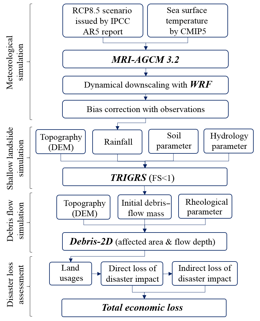
Based on the above description, a potential method for predicting the impact of climate change on slope land was to link climate scenarios, landslide prediction, debris-flow transport simulation with their consequent direct and indirect loss assessment. The model selection and simulation process were introduced step by step below.

2.1 Scenarios and models

In recent decades, the climate projections for various periods have been widely studied using general circulation models (GCMs). However, the resolution of GCMs is insufficient to simulate data for further application in hydrology or agriculture at the local level. For example, in typhoon-related rainfall, GCM results cannot provide details on weather patterns in the local area. Furthermore, it is not possible to obtain assessments on a daily or hourly basis. To link the simulations of atmosphere and hydrology, downscaling techniques (statistical or dynamic downscaling) are useful. In Taiwan, these techniques have been applied to climate projection simulations by the Taiwan Climate Change Projection and Information Platform (TCCIP) funded by the Ministry of Science and Technology, and the downscaling data set is freely available on their official website (TCCIP, 2017). For the data provided by TCCIP, the atmospheric general circulation model 3.2 (AGCM 3.2), developed by the Meteorological Research Institute (MRI), Japan Meteorological Agency (JMA), is used for global climate simulation at a 20 km horizontal resolution (Mizuta et al., 2012). The observed sea surface temperatures are considered as lower boundary conditions by the Coupled Model Intercomparison Project Phase 5 (CMIP5). Using the initial boundary conditions specified by the results from MRI-AGCM 3.2, the dynamic downscaling data set at a 5 km horizontal resolution is simulated by the Weather Research and Forecasting (WRF) modelling system (Skamarock et al., 2008) developed by the US National Center for Atmospheric Research (NCAR). Because errors in the estimation of total rainfall are still found in the WRF results, the quantile mapping method is adopted for bias correction in these data sets (Su et al., 2016). The rainfall scenarios in this study were directly collected from TCCIP.

The potential landslide simulation model is used to evaluate the probability of landslides. It encompasses two major approaches: statistical and physical. The common statistical approach employs a regression model, such as binary regression, to identify a set of maximum likelihood parameters based on historical data to predict the landslide distribution (Chang and Chiang, 2009). In the physical approach, the infinite slope stability theory is applied to calculate the safety factor and predict the potential landslide area, such as the Transient Rainfall Infiltration and Grid-based Regional Slope-Stability model (TRIGRS) (Baum et al., 2008) and a digital terrain model for mapping the pattern of potential shallow slope instability (SHALSTAB) (Montgomery and Dietrich, 1994). Because the rainfall input in each grid cell is non-homogeneous over space and time, a grid-based model could be practically useful for establishing the connection between rainfall and landslides. In this study, a physical approach using the TRIGRS model was selected to forecast shallow landslide occurrence under rainfall events.

For debris flow assessment, the empirical formula (Ikeya, 1981) has been resorted to. However, in recent years, because of the progress made in computer technology, numerical simulation has turned out to be a powerful approach. Various kinds of useful numerical programmes have been developed by research and academic institutions worldwide. Although they are based on different theories, the governing equations are derived from mass and momentum conservations (Hutter and Greve, 2017; O'Brien et al., 1993; Hungr, 1995; Sassa et al., 2004; Liu and Huang, 2006; Nakatani et al., 2008; Armanini et al., 2009; Christen et al., 2010). According to the practical application of inputs, the models can be divided into hydrological- and geologic-based models. In hydrological-based models, the debris flow is simulated with a calibrated hydrograph at a specified inflow location, and it is particularly applied to channelized debris flows or mud flows. However, in the geologic-based models, debris flow starts from an initial mass distributed in its source areas, such as landslide-triggered debris flow or an avalanche. To link the debris flow simulation with the landslide results, a geologic-based model is more useful. Among different models, the Debris-2D (Liu and Huang, 2006) has been widely applied and validated in different cases in Taiwan (Liu et al., 2009, 2013; Tsai et al., 2011; Wu et al., 2013) and is especially suitable for landslide-triggered debris flows (Wu et al., 2013). Hence, in this study, we used the Debris-2D to simulate the debris flow transport process.

Table 1 Property loss function of slope land disasters.

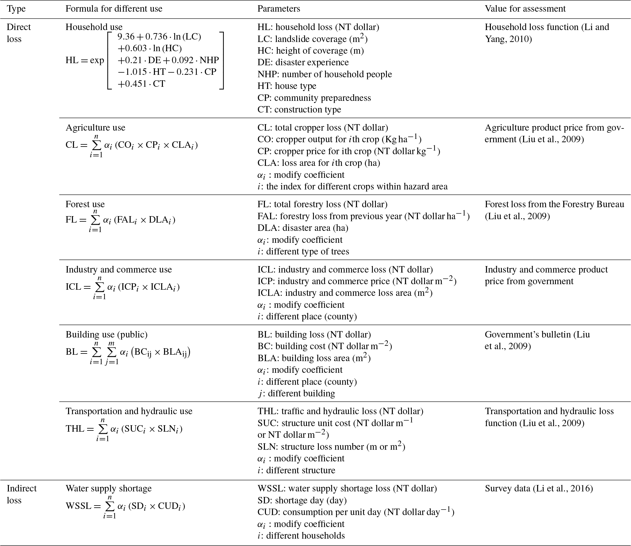
Conventionally, slope land losses are divided into direct and indirect losses. For assessing the direct loss from the debris flow disasters in Taiwan's mountainous regions, a method was devised by Liu et al. (2009). The major losses that are assessed include construction, agriculture, forest, transportation, hydraulic, and tourism losses. Li and Yang (2010) built a household loss regression model for debris flow depending on actual survey data. This model considered several statistically significant variables, including the coverage area, the height of debris flow coverage, number of people per household, and type of construction material (RC), to assess the actual household loss incurred from the debris flow.

Based on experience from historical typhoon events, the major indirect impact of slope land disasters on Taipei is water shortages. This study emphasized the economic effects of water supply disruption. According to the questionnaire survey of Typhoon Soudelor (Li et al., 2016), 54.7 % of all Taipei households (approximately 1 million) were affected by the disrupted water supply resulting from high turbidity. The average economic loss per household caused by water supply shortage is USD 100. The majority of this expenditure was to buy clean drinking water; people also had to spend on water for routine cleaning and washing. This study evaluated the water supply shortage (based on the survey data of Typhoon Soudelor), including the percentage of affected households in Taipei and the loss faced per household. All methods of quantifying losses are listed in Table 1, and the ensuing loss assessment of slope land disasters is based on this table.

2.2 Integrated simulation process

An integrated simulation process was constructed as depicted in Fig. 1. The rainfall events were simulated using MRI-AGCM 3.2, downscaled with WRF, and modified by bias correction. To accomplish the study's objectives regarding climate change and its impacts, the simplest method is to study two extreme rainfall scenarios from different periods and compare them. This scenario approach was adopted for integrated simulation. According to the Representative Concentration Pathway 8.5 (RCP 8.5) scenario issued by the IPCC fifth assessment report (AR5), the projected rainfall data in the late 20th (1979–2003) and 21st centuries (2075–2099) were simulated from TCCIP, and the hourly rainfall at 5 km horizontal resolution is provided for the end user. However, this resolution is inadequate for the simulation of landslides or debris flow. In landslide and debris flow simulation, the typical 40 m × 40 m DEM was used as topography input. To satisfy the spatial resolution of 40 m × 40 m, the rainfall was interpolated by inverse distance weighting (IDW) method from 5 km × 5 km to 40 m × 40 m.

Figure 1 Integrated simulation process.

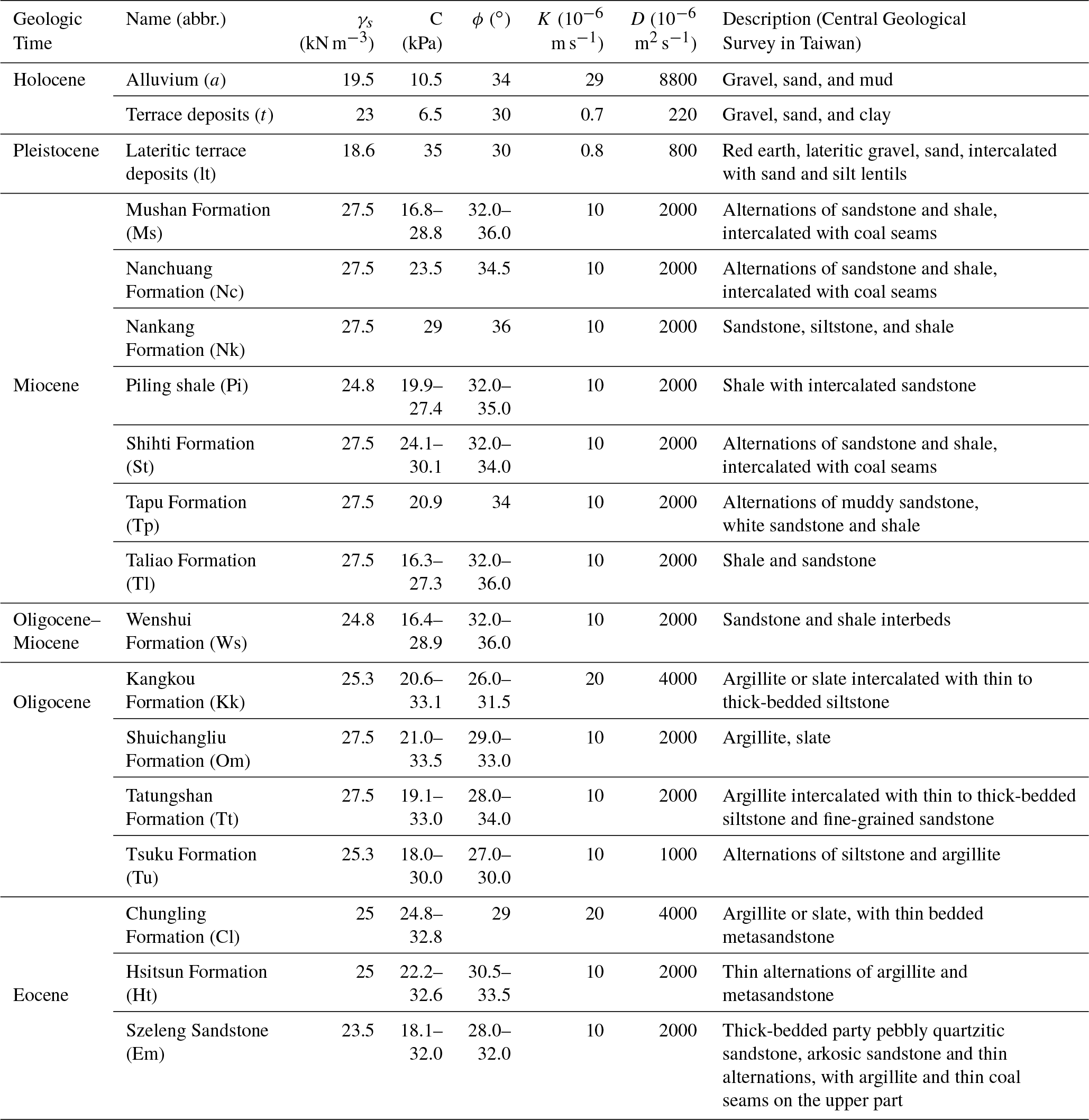
To determine the unstable slope under rainfall scenarios, the TRIGRS was used to simulate the factor of safety (FS) on each grid. In the TRIGRS simulation, the input data of each grid cell is separated into four parts: rainfall intensity, topographic information, soil, and hydraulic parameters. The rainfall intensity I_nZ (mm hr⁻¹) presented in the previous paragraph was directly used. The topographic information, such as slope and flow aspect, were derived from DEM at a 40 m resolution. The soil thickness d_LZ was determined with an empirical slope-depth classification based on the survey data in Taiwan (Chen et al., 2010), as shown in Table S1 in the Supplement. The soil parameters of cohesion C, friction angle ϕ, and unit weight γ_s were calibrated based on past events. The hydraulic parameters of saturated conductivity K_S and diffusivity D₀ for the various geologic conditions could be calibrated or cited from past investigations. Without considering antecedent precipitation, the initial depth of the steady-state water table d was assumed to be the same as that of the soil thickness d_LZ, and the initial infiltration rate for soil was taken to be 10⁻⁸ (m s⁻¹) (Chen et al., 2005).

To calibrate parameters more accurately, we defined different zones based on geologic setting and historical landslide rate. In each defined zone, the modified success rate (MSR) provided by Huang and Kao (2006) was used for calibration and validation parameters, as shown below:

$$\begin{array}{}\text{(1)}& \mathrm{MSR}\left(\mathit{\%}\right)={\displaystyle \frac{\mathrm{1}}{\mathrm{2}}}{\displaystyle \frac{N_{\mathrm{1}}}{N_{\mathrm{1}}+N_{\mathrm{2}}}}+{\displaystyle \frac{\mathrm{1}}{\mathrm{2}}}{\displaystyle \frac{N_{\mathrm{4}}}{N_{\mathrm{3}}+N_{\mathrm{4}}}},\end{array}$$

where N₁ and N₂ denote the areas of FS<1 and FS>1, for the historical landslide areas. Similarly, N₃ and N₄ represent the areas of FS<1 and FS>1 for the historical non-landslide areas. The success rates of landslides and non-landslides can be obtained using Eq. (1). The units N₁−N₄ were calculated from the slope units. The successful calibration and validation is considered if the MSR>70 %.

With the aid of rainfall and other calibrated parameters, the FS was simulated using TRIGRS. At the beginning of the TRIGRS simulation, the FS of each grid is larger than 1; specifically, the infinite slope is stable at the beginning. With the onset of rainfall and infiltration, the FS decreases because of an increase in the pore water pressure. Grid instability or infinite slope failure occurs when the FS is less than 1, and it is regarded as a potential shallow landslide area. The potential shallow landslide volume or mass of the initial debris flow could be further evaluated for the debris flow simulation using the soil thickness d_LZ in each unstable grid.

Under extreme rainfall and loose shallow landslide mass, sediment transport by debris flow from the upstream catchment was assumed. Accordingly, all shallow landslide masses were considered as the input of debris flow and simulated using Debris-2D. In Debris-2D simulation, the input data are topography, initial debris flow depth H, and yield stress τ₀. The topography using the digital elevation model (DEM) is the same as using a TRIGRS input. With the potential shallow landslide area simulated by TRIGRS and its corresponding soil thickness d_LZ in each unstable grid, the initial debris flow depth H can be determined by a simple relation (Liu and Huang, 2006; Liu et al., 2009):

$$\begin{array}{}\text{(2)}& H=d_{\mathrm{LZ}}/C_{d\mathrm{\infty }},\end{array}$$

where C_d∞ is the equilibrium concentration (Takahashi, 1981), which is calculated as follows:

$$\begin{array}{}\text{(3)}& C_{d\mathrm{\infty }}={\displaystyle \frac{\mathit{\rho }\tan \mathit{\theta }}{\left(\mathit{\sigma }-\mathit{\rho }\right)\left(\tan \mathit{\varphi }-\tan \mathit{\theta }\right)}},\end{array}$$

where ρ and σ are the densities of water and sediment, ϕ is the internal friction angel, and θ is the average creek bottom slope. For the yield stress τ₀, it can be obtained by samples collected from the field (Liu and Huang, 2006).

In reality, the landslide-triggered debris flows in different locations could occur at different times. However, the occurrence of debris flow after slope failure could not be predicted so far, and what we are concerned with in this paper is the final volume and influence area caused by debris flows. Hence, we assumed all debris flows started up at the same time and this assumption has no effect on the final result.

The debris flow coverage area will be intersected with the land-use map to identify the loss of different uses (e.g. household use, agriculture use, and forest use). The economic losses incurred from the slope land disaster were evaluated by loss functions and the corresponding parameters established in the database according to the uses. The total losses are the summation of the individual losses in different uses.

The integrated simulation in Fig. 1 provided a comprehensive view of the chain reaction. The simulation results from the current and future scenarios were compared in terms of climate change, and the compounded disasters were calculated for the extreme climatic events.

3 Case study: Xindian watershed

3.1 Study area

Xindian watershed is located upstream of the city Taipei in northern Taiwan. The river is one of the three major tributaries of the Tamsui River, and it is also the main source of drinking water for Taipei and New Taipei cities. According to the Taipei City Running Water Center, over 1 million Taipei households rely on this river for their drinking water requirements. The chief tributaries of the Xindian River are Nanshi and Beishi, represented in Fig. 2. Comparing these two tributaries, the Nanshi River catchment area is more fractured than the Beishi River catchment, and historically, landslides were rampant along the Nanshi River (Fig. 3). Hence, in this study, we focused on the Nanshi River catchment and ignored the areas beyond the Feitsui Reservoir.

Figure 2 Topography (shaded relief) and location of the study area.

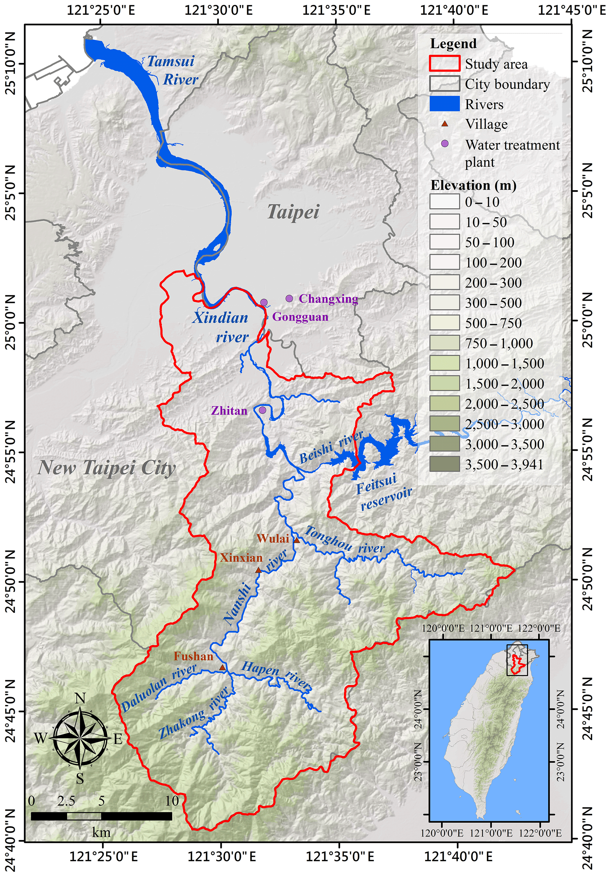
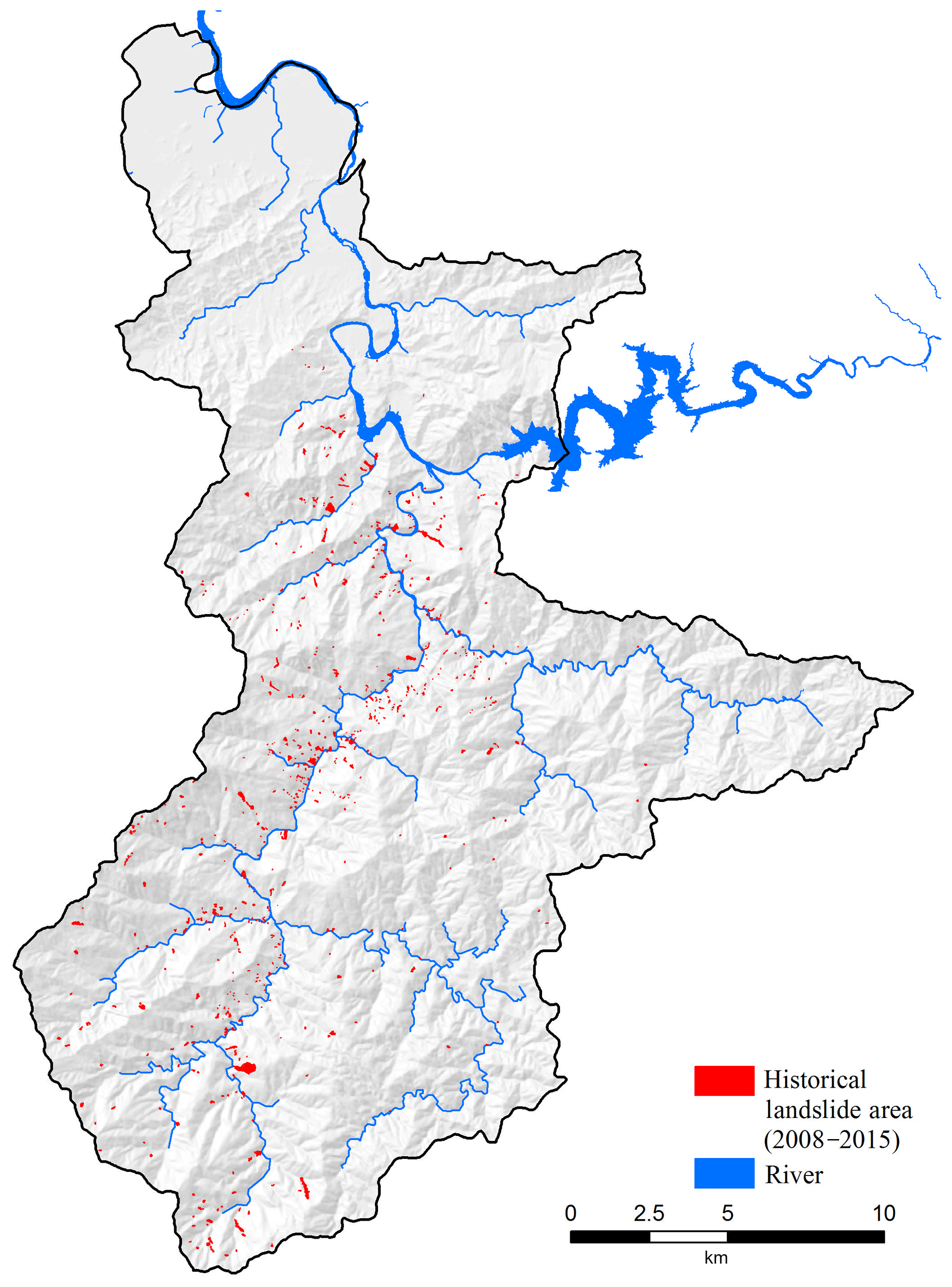
Figure 3 Historical landslide area delineated by aerial photos annually from 2008 to 2015 (source: Central Geological Survey, Taiwan).

The study region depicted in Fig. 2 spans an area of 49 000 ha. Villages such as Wulai, Xinxian, and Fushan are located along the Nanshi River with 2716, 622, and 739 inhabitants, respectively. In this area, the elevation varies considerably and canyon-like topography can be noticed along the banks of the river. The study area is mainly located in the Tatungshan (Tt), Szeleng Sandstone (Em), Kangkou (Kk), Mushan (Ms), and Tsuku formations (Tu). Its contents include sandstone, argillite, slate, shale, and siltstone, represented in Fig. 4. The age of the geological setting is between the Holocene and Eocene epochs. Numerous folds and faults occur in this region. Because of the soft and fractured geological conditions prevailing in the Nanshi River catchment, geo-disasters and the resultant sedimentation are major concerns in the area.

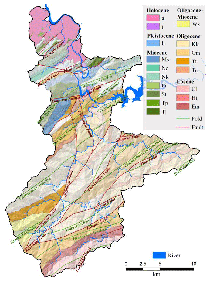
Figure 4 Lithological map – 1 : 50 000 scale; the abbreviations in the legend are listed in Table 3.

Considering the above-mentioned facts, the Xindian watershed is an appropriate area for studying the impacts of slope land hazards. The economic impacts of sediment-related hazards are not only restricted to this area but also felt in the downstream cities, particularly in Taiwan's capital. For long-term city planning, it is of utmost importance to comprehend the whole situation and devise suitable strategies, after due consideration of climate change aspects. Accordingly, the integrated simulation built in the previous section was used to analyse the area. The model calibration and simulation results are presented in the following sections.

Figure 5 Top 20 rainfall events of the late 20th and 21st centuries.

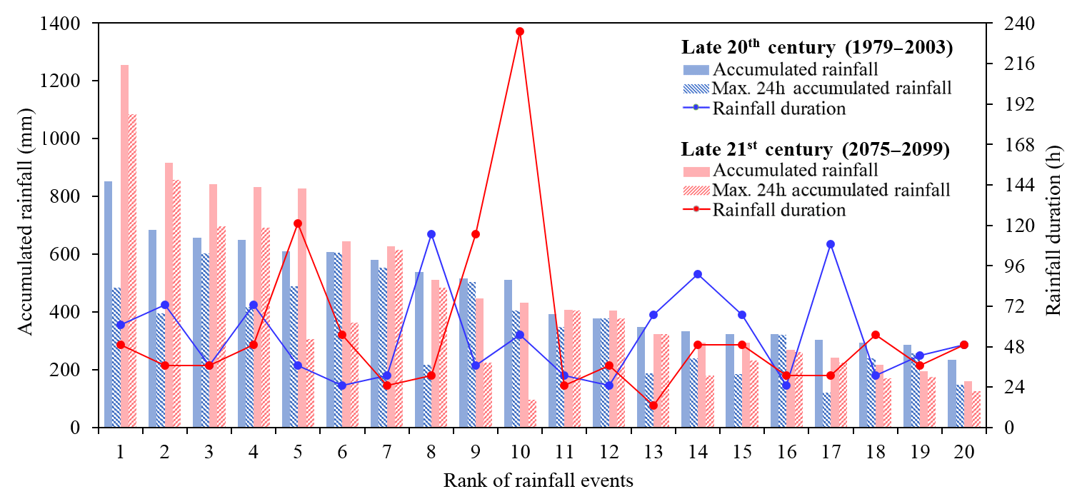
Figure 6 Accumulated rainfall distribution (a: rank 1 rainfall of the late 20th century, b: rank 1 rainfall of late 21st century).

3.2 Extreme rainfall scenarios

The rainfall projections for the late 20th (1979–2003) and 21st centuries (2075–2099) collected from TCCIP were chosen for comparison in our study area. The top 20 rainfall events of the late 20th and 21st centuries are presented in Fig. 5. A pattern of increasing rainfall can be observed in the top five rainfall events.

To explore the potential impacts of the slope land problem in extreme climatic conditions, the worst cases (rank one rainfall event) from the late 20th and 21st centuries were selected for comparison. They are referred to as scenario 1 and scenario 2 in the following discussion. For both scenarios, the temporal and spatial resolutions were 1 hr and 5 km. As mentioned in Sect. 2.2, the IDW interpolation was adopted and the spatial resolution was downscaled from 5 km to 40 m to fit the DEM.

The distribution of the accumulated rainfall for both scenarios is shown in Fig. 6. Based on data provided by the Fushan meteorological station, the maximum accumulated rainfall was 911.4 mm in 61 h and 1531.1 mm in 40 h for scenario 1 and scenario 2, respectively. Similarly, the maximum intensities were 49.7 and 125.8 mm hr⁻¹.

Table 2 Calibration and verification of the TRIGRS model based on MSR calculation.

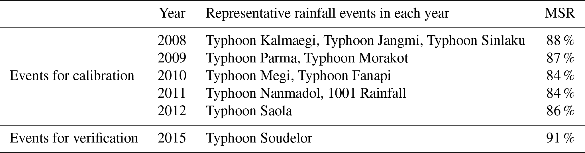
Table 3 The geology description and corresponding parameters used in TRIGRS.

3.3 Shallow landslides simulation

In TRIGRS simulation, the required input data were soil and hydraulic parameters. The hydraulic parameters of saturated conductivity K_S and diffusivity D₀ for the various geologic conditions were cited from past investigations (Central Geological Survey, 2010), as shown in Table 4. The soil parameters of cohesion C, friction angle ϕ, and unit weight γ_s are subject to geological changes and historical landslide rate. In the study area, there are 18 geologic settings (Fig. 4) and we used five classes to define different calibration zones on each geologic setting based on the ratio of historical landslides in each slope unit; i.e. there are 90 zones for parameters calibration. However, some geologic settings are stable without landslides. So the total number of zones decreases to 56 for parameter calibration. With the objective function of MSR (Eq. 1), the parameters in each zone could be optimized for the rainfall events provided by the Central Weather Bureau and the historical landslide data provided by the Central Geological Survey (Fig. 3). However, the historical landslide data are only updated annually; hence, the sum of representative rainfall events each year was used for calibration. The landslide of Typhoon Soudelor in 2015 was successfully validated with an MSR of 91 %; the calibration and validation results are presented in Table 2 and the calibrated parameters are listed in Table 3. Therefore, the predictions of the landslide model for the study area were accurate.

In the simulation of these two scenarios, an increasing trend was observed in the potential landslide areas, in terms of the accumulated rainfall with a time delay. Moreover, the rate of increase in the accumulated landslide ratio in scenario 2 was found to be higher than in scenario 1, which could be attributed to the effect of rainfall intensity, as illustrated in Fig. 7. The stable time periods with maximum accumulated landslide ratios for scenario 1 and scenario 2 were 65 and 40 h. Based on the landslide simulation results, the potential shallow landslide area (FS<1) is depicted in Fig. 8. The output data of landslide area by TRIGRS and the estimated soil thickness d_LZ based on slope angle would be the input data of Debris-2D for simulating the debris flow volumes.

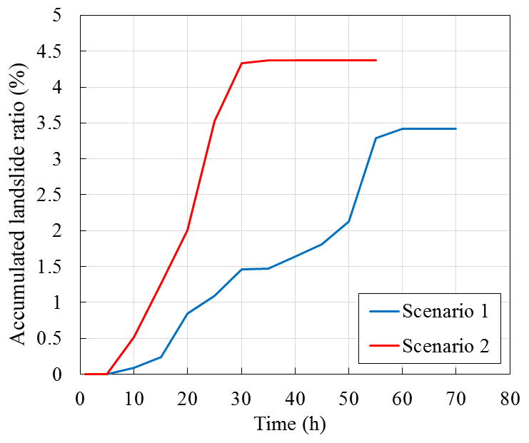
Figure 7 Accumulated landslide ratio vs. time for scenarios 1 and 2 (landslide rate was calculated using the area of FS < 1 over the whole area of the watershed).

Table 4 Comparison of rainfall and debris flow volume.

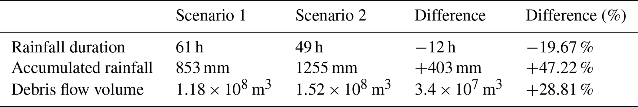
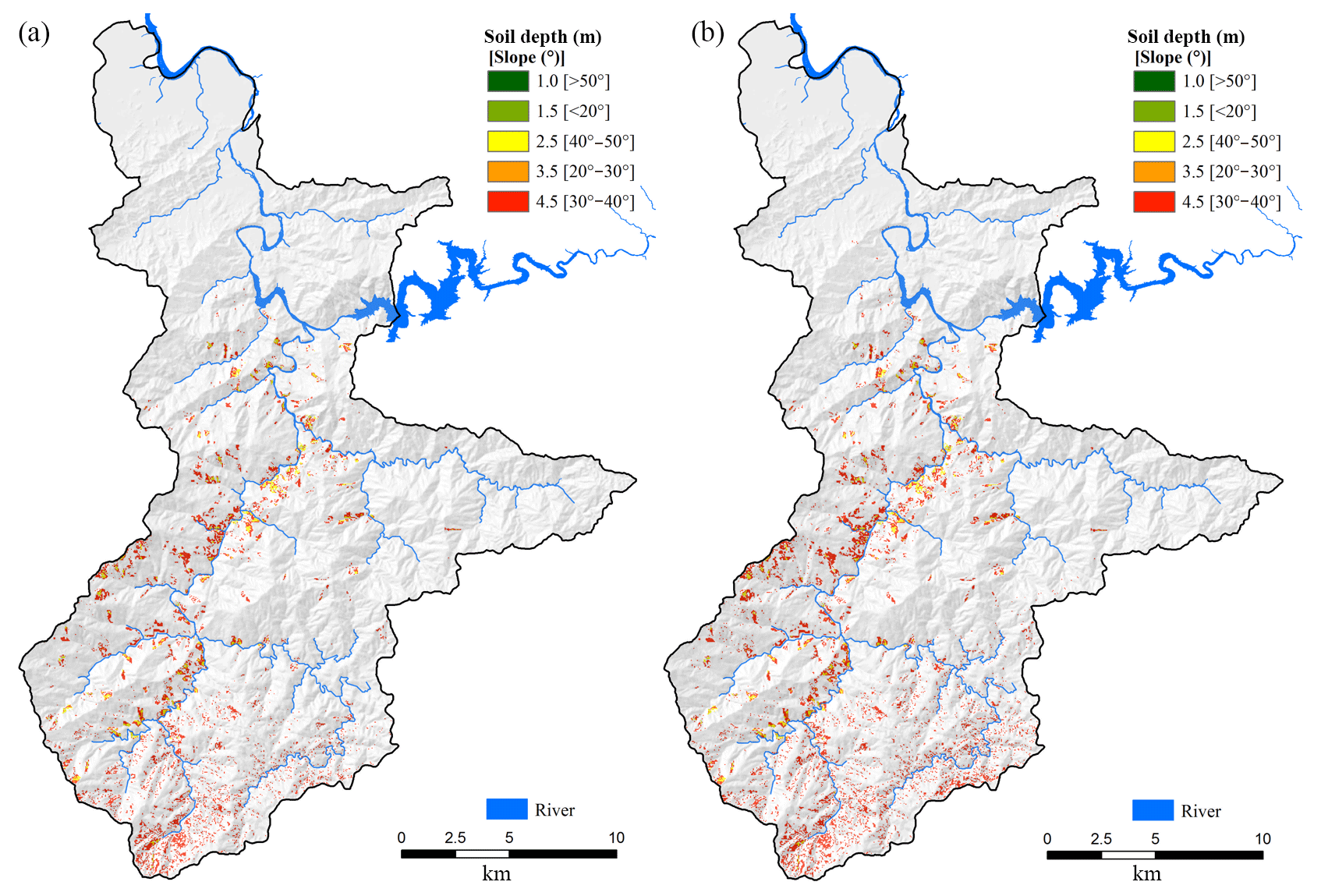
Figure 8 Shallow landslide area simulated by TRIGRS with input soil depth classified by slope angle (a: scenario 1, b: scenario 2).

3.4 Debris flow simulation

In Debris-2D simulations, we have to find the initial debris flow mass and rheological parameters. To calculate the initial debris flow mass, potential shallow landslide area and soil depth (Fig. 8) were used, as well as Eqs. (2) and (3). The equilibrium concentration of debris flow in Eq. (2) can be estimated by an empirical formula purposed by Takahashi (1981) in Eq. (3) and the maximum value cannot exceed 0.603 (Liu and Huang, 2006), which occurred when the slope was larger than 20.6^∘. Due to the slope of our study basin being even larger than 20.6^∘, this paper took 0.603 as the concentration value of the debris flow to estimate debris flow volumes in Eq. (2). The rheological parameter yield stress was estimated to be 800 Pa (Geotechnical Engineering Office, 2011) and was used in subsequent simulations.

The depth of debris flow in both scenarios is presented in Fig. 9 and its characteristics are described as follows. At a simulation time of 5 min, the flow depth was over 20 m, and it occurred in the Zhakong River and in the midstream of the Nanshi River. The source of the debris flow in the Zhakong River was an upstream landslide. However, the debris flow that occurred in the midstream of the Nanshi River originated from the left bank landslide along the same river. At 10 min, all landslide debris was flowing into the nearby tributary. In scenario 2, the front of the Zhakong River debris flow reached the tail end of the Nanshi River debris flow at 15 min. After 20 min, the downstream Hapen River debris flow converged toward the Zhakong River debris flow. All debris flows started to decelerate and stopped completely at 30 min.

In both scenarios, the upstream Hapen River debris flows could not be transported downstream because of the meandering creek. The landslide debris along the downstream Hapen and Daluolan rivers were mainly deposited at the junction of the Zhakong, Daluolan, and Happen rivers. The depths of the Daluolan and Happen rivers made them insusceptible to the debris flow from the Zhakong or Nanshi rivers. The front of the Zhakong River debris flow was deposited ahead of a sharp turn upstream of the Nanshi River in scenario 1, but it managed to reach the tail end of the Nanshi River debris flow in scenario 2. The Nanshi River debris flows were deposited at the junction of the Nanshi and Tonghou rivers.

4 Results and discussion

4.1 Potential effects on natural hazards

In scenarios 1 and 2, the grid-averaged maximum accumulated rainfalls were 853 mm in 61 h and 1255 mm in 49 h. Comparing the two scenarios, the grid-averaged accumulated rainfall was observed to increase by 402 mm, but the duration decreased by 12 h. Based on scenario 1, the decrement in duration and increment in grid-averaged accumulated rainfall between the two scenarios were 19.67 % and 47.22 %. Hence, the characteristic of the rainfall changed to a shorter duration and greater intensity.

For the two rainfall scenarios, the total volumes, including landslide and debris flow volumes, calculated from Eq. (1) were 1.18×10⁸ m³ and 1.52×10⁸ m³. The incremental volume between the two scenarios was 28.81 %.

Figure 9 Final flow depth of debris flow simulated by DEBRIS-2D (a: scenario 1, b: scenario 2).

Figure 10 Direct losses.

Figure 11 Indirect losses.

4.2 Loss assessment for compounded disasters

Based on the debris flow coverage area, possible economic losses in different land uses were evaluated according to the quantified method of disaster loss in Table 1. The direct and indirect losses were determined in Table 5 and illustrated in Figs. 10 and 11.

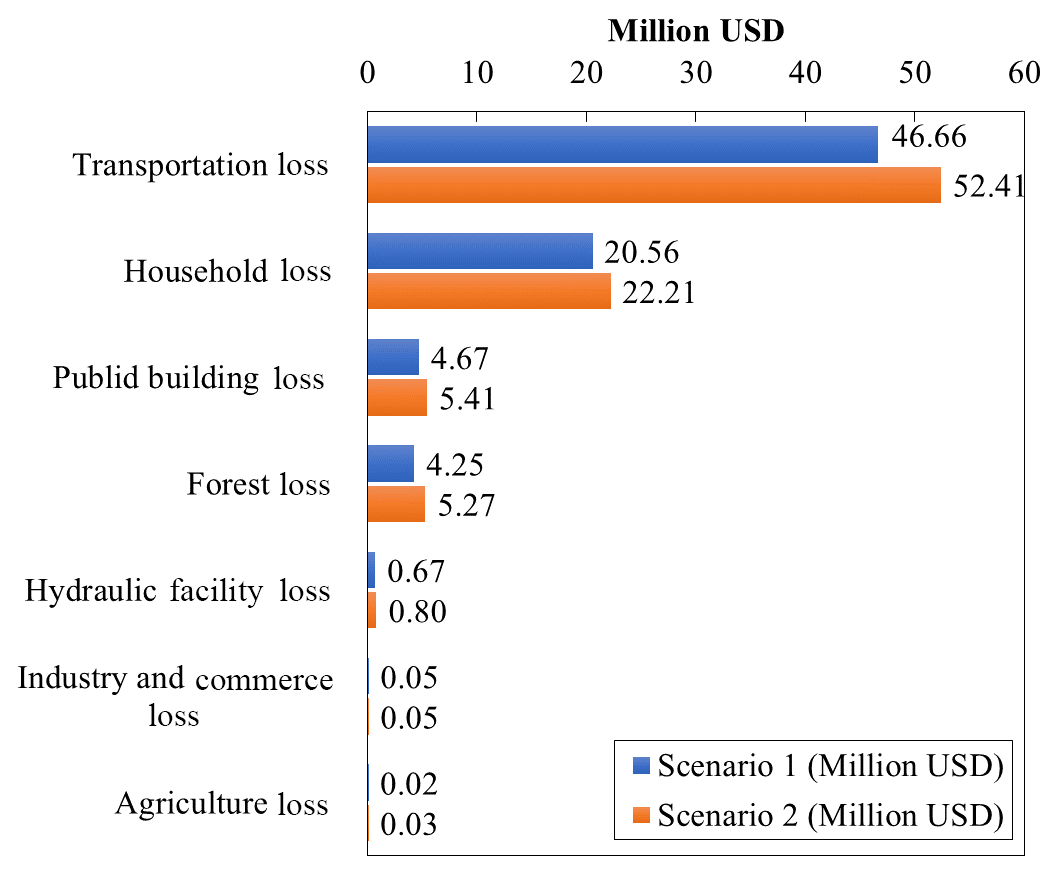
According to Fig. 10, the main direct losses were to transportation, households, and public facilities. Because most of the roads were built along the riverside, they were easily damaged by the landslide and debris flow. This transportation loss constituted the biggest impact of the disaster, as witnessed in Fig. 10. The transportation losses in scenario 2 were even more severe than in scenario 1, amounting to 12.32 % and approximately USD 52.14 million. The second largest was household losses; affected households were predominantly located along the riverside. In this case too, the losses in scenario 2 were more severe than in scenario 1, amounting to approximately 8.01 % and USD 22.21 million. The third largest loss was faced by public facilities, including power supply, water supply, hospitals, and schools.

Table 5 Comparison of economic losses.

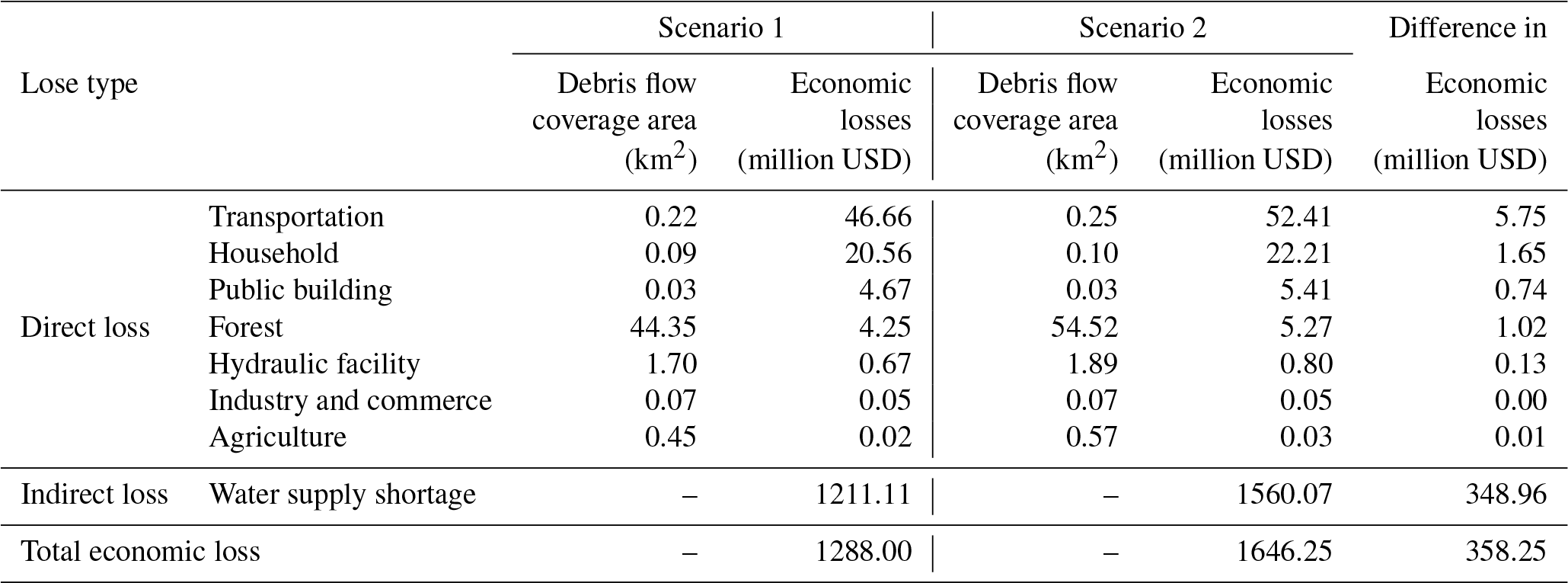
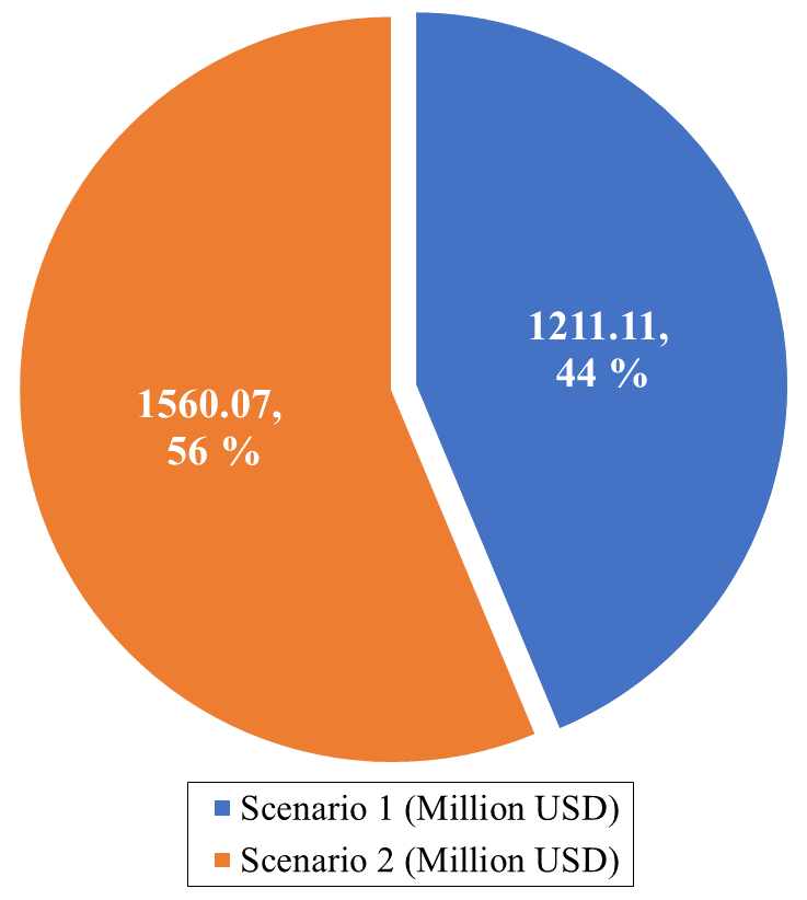
Among the indirect losses, this study mainly focused on water supply shortage. According to the household survey data of Typhoon Soudelor in 2016 (Li et al., 2016), 54.7 % of Taipei households were affected by turbid water caused by the landslide that occurred upstream. The total landslide volume was estimated to be 9.8×10⁶ m³ (Wu et al., 2016a) and caused water supply shortages for 42 h. Therefore, compared with the debris flow volume in Table 4, the volumes in scenarios 1 and 2 were 12 and 15.5 times greater than Typhoon Soudelor. Because the capacity of water treatment plants to remove turbidity is fixed, the required treatment time for turbid water is proportional to the debris flow volume. Based on the comparison of the landslide volume with the Typhoon Soudelor, the water supply shortage time periods in scenarios 1 and 2 were 506 and 651 h. Therefore, the total economic losses were evaluated to be USD 1211.11 million and USD 1560.07 million, as depicted in Fig. 11.

Table 5 lists the total losses (direct and indirect) incurred in scenarios 1 and 2. Accordingly, the total loss faced in scenario 2 was approximately USD 1646.25 million, which is greater than the USD 1228.00 million loss faced in scenario 1. In other words, increased precipitation triggered by extreme events related to climate change is likely to cause more damage in the future than at present, and the losses are projected to increase by 27.8 % or USD 358.25 million.

Furthermore, another problem worthy of discussion is that the indirect losses in scenarios 1 and 2 are both far greater than the direct losses. This means that the indirect losses are more damaging than the direct losses, and the ratios (indirect loss divided by direct loss) for scenarios 1 and 2 were calculated to be 15.75 and 18.1. In addition, the results substantiated that more serious disasters result in a higher proportion of indirect losses. Therefore, when discussing climate-induced slope land impacts faced by Taipei, considering only direct losses will result in grossly underestimating the actual magnitude of the impact.

5 Conclusions

In recent years, slope land problems associated with climate change have become crucial topics of discussion. With the aid of projected climate scenarios, an integrated physical simulation process was proposed for analysing the potential impacts from a watershed point of view. The Xindian watershed in Taiwan was selected to study the effects of extreme rainfall events. Shallow landslides, debris flow, and related loss assessments were executed in a step-by-step manner.

The rainfall scenarios in the late 20th (1979–2003) and 21st centuries (2075–2099) were simulated using MRI-AGCM 3.2, and dynamic downscaling with WRF was adopted to produce the hourly rainfall data in a 5 km horizontal resolution. The resulting data were further interpolated using the IDW method from 5 km to 40 m for the shallow landslide simulation input. The potential shallow landslide area was varied according to the changing rainfall and was simulated using the TRIGRS model, which was calibrated and validated based on past events. Later, the corresponding debris flow volume was determined using the equilibrium concentration, and the debris flow was simulated with the help of the Debris-2D model. With the aid of these simulation results, multiple loss functions were used to evaluate direct and indirect economic losses.

Upon comparing the worst cases of rainfall in the late 20th and 21st centuries, the grid-averaged accumulated rainfall increased by 47.22 %, but the duration decreased by 19.67 %. Considering the increased rainfall intensity in scenario 2, the estimated volume caused by the chain impacts of shallow landslides and debris flow was increased by 28.81 %. Because of the increasing impacts of slope land disasters caused by climate change, the economic losses are projected to increase by 27.8 % or USD 358.25 million. Among all of the losses, the main direct losses were to transportation, households, and public facilities in mountainous areas; the chief indirect loss was the water supply shortage in urban areas. Notably, the value of the indirect losses in both scenarios was much greater than that for the direct losses. This means that, whenever heavy rainfall causes slope land disasters in areas other than the Taipei Metropolitan Area, its influence on Taipei will be mainly in the form of indirect impacts. This study solely discussed the problem of a water supply shortage in residential areas. If industrial and commercial losses are also included, the economic impacts will be increased manifold. Therefore, methods to improve the resilience of water resources, as well as the development of alternative water sources (such as establishing cross-regional water transfer mechanisms and groundwater wells), will be crucial adaptation strategies for the Taipei Metropolitan Area in response to slope land disaster impacts resulting from climate change.