Recent Baltic Sea storm surge events from a climate perspective

Three storm surge events with return periods between 10 and 100 years have occurred in the western Baltic Sea in recent years (2017, 2019 and 2023). While in most cases such surge events are associated with high wind speeds, two of the three events occurred at relatively moderate wind speeds. The events are analysed and decomposed into the contributions from different factors, such as direct atmospheric effects or prefilling of the Baltic Sea, which can lead to such extreme water levels. A numerical hindcast is used to place the events and their contributing components into a climate perspective. While the absolute water levels were among the highest in recent decades, the individual contributions of the direct atmospheric effects as well as prefilling were not unusual for two of the three events and rather a combination of atmospherically induced water level changes and prefilling caused such prominent extreme events. Although the perceived increased frequency of the events may indicate a relation to climate change, the individual contributions were within the range of climate variability observed in recent decades.

1 Introduction

Storm surges are the primary cause of coastal flooding along the world's low-lying coastlines (Bernier et al., 2024). In the Baltic Sea, where amplitudes of astronomical tides are small everywhere, considerable storm surge heights can occur and pose a threat, in particular in the southwestern regions (Wolski et al., 2014; Aakjær and Buch, 2022; Hofstede and Hamann, 2022; Kiesel et al., 2024), the Gulf of Finland (Suursaar and Sooäär, 2007; Averkiev and Klevannyy, 2010), the Gulf of Riga (Suursaar et al., 2006; Suursaar and Sooäär, 2007; Männikus et al., 2019) or the Gulf of Bothnia (Averkiev and Klevannyy, 2010).

In recent years, three very severe storm surge events have been observed in the southwestern part, mainly affecting the German and the Danish coastlines. The first event occurred on 4–5 January 2017 and caused peak water levels of about 1.39 to 1.83 m (BSH, 2017) above the mean water level (MWL) along the German Baltic Sea coast (Fig. 1). This event was ranked under the five highest surges since 1950 at most gauges on the German Baltic Sea coast (Liu et al., 2022; https://stormsurge-monitor.eu, last access: 25 June 2025). The second event occurred on 2 January 2019 and caused water levels between 1.41 and 1.91 m (BSH, 2019) along the coast. In Warnemünde, the maximum water level reached during the event was close to the highest observed since 1954 (Liu et al., 2022). Finally, on 20 October 2023, a severe storm surge event led to water levels from 1.08 to 2.27 m along the German coast (BSH, 2023). It caused widespread flooding in cities such as Flensburg and Schleswig (Germany), led to the breaching of at least seven (regional) dikes, and caused damages of more than EUR 200 million in Schleswig-Holstein (Kiesel et al., 2024).

While all events were characterized by high surges, the meteorological and oceanographic situation differed. The event in 2017 occurred at relatively low wind speeds and was referred to as a “silent storm surge” in the literature (She and Nielsen, 2019). Wind speeds during the 2019 event were higher but still not extreme over the southwestern Baltic Sea. Finally, during the event in 2023 strong easterly winds persisted for 2 d and reached peak wind speeds of 102 km h⁻¹ (Kiesel et al., 2024).

While strong onshore winds are the primary cause for coastal storm surges, there are other factors that may substantially enhance coastal sea levels. Such factors vary from region to region. The Baltic Sea is a semi-enclosed sea that is connected to the North Sea only through the relatively narrow Danish Straits. During periods of the prevailing westerly winds the sea level gradient across the Danish Straits increases, leading to higher inflow and higher Baltic Sea water volumes (Samuelsson and Stigebrandt, 1996). Transports across the Danish Straits can reach values of up to about 45 km³ d⁻¹ in both directions, which corresponds to a sea level change of about 12 cm d⁻¹ over the entire Baltic Sea (Mohrholz, 2018). Typically, such variations that may lead to a prefilling (Lehmann and Post, 2015; Andrée et al., 2023) of the Baltic Sea have timescales of about 8 d (Soomere et al., 2015) or even longer, from weeks to even a month in some cases (Soomere and Pindsoo, 2016). They may substantially enhance the mean water level before the onset of a storm (Suursaar et al., 2006; Madsen et al., 2015). As a consequence, similar storms may lead to different water levels depending on prefilling.

Atmospheric variability on timescales shorter than about 10 d may lead to a redistribution of water masses within the Baltic Sea basin (Kulikov et al., 2015) or between the Baltic proper and the Gulf of Riga (Männikus et al., 2019). In addition, seiches with periods of up to tens of hours and e-folding times of up to 2 d may develop (Leppäranta and Myrberg, 2009), the details of which are still debated and are still not fully understood (e.g. Wübber and Krauss, 1979; Otsmann et al., 2001; Jönsson et al., 2008). When unfavourably coupled with storm surges or in resonance with atmospheric forcing, such oscillations may contribute to very high sea level extremes on the coast (Suursaar et al., 2006; Weisse and Weidemann, 2017; Wolski and Wiśniewski, 2020).

The three very severe storm surge events affecting the southwestern Baltic Sea in 2017, 2019 and 2023 occurred at different wind speeds. It is therefore obvious that other factors must have contributed differently to the severity of the storm surges. While the individual events were to some extent discussed in the literature (e.g. Suursaar et al., 2006; She and Nielsen, 2019; Aakjær and Buch, 2022; Kiesel et al., 2024), a systematic assessment and comparison of the events are lacking.

In this study, we aim at such a comparison from a climate perspective. Using data from a 1958–2023 hydrodynamic hindcast (Weidemann, 2015) we first decompose the three events and analyse the extent to which different factors such as prefilling have contributed and may account for the observed differences. Based on the multidecadal hindcast we subsequently derive a climatology and assess the extent to which these events have been unusual.

2 Data and methods

2.1 Numerical model data

To analyse water levels from 1958 to 2023, an existing hindcast by Weisse and Weidemann (2017) is used for the period 1958–2011 and extended from 2012 to 2023. For the extension, the same model set-up was used to achieve the best possible homogeneity. For the hindcast and its extension, the hydrodynamic model TRIM-NP (Casulli and Stelling, 1998; Kapitza and Eppel, 2000; Kapitza, 2008) in barotropic mode was used with a triple-nested grid. The coarsest grid covers the northeastern Atlantic with a resolution of 12.8 km, and the finest nest covers the southwestern Baltic Sea with a resolution of 1.6 km (Fig. 1).

Just as with the existing water level hindcast (Weisse and Weidemann, 2017), for the years 2011 to 2023 the model was forced by atmospheric conditions from an extension of the COSMO-CLM atmospheric hindcast simulation (coastDat2, coastDat3) (Geyer, 2014). This atmospheric hindcast covers the EURO-CORDEX domain (Kotlarski et al., 2014), has a spatial resolution of about 22 km and is driven by the global NCEP reanalysis (Kalnay et al., 1996) at its lateral boundaries. In addition, a spectral-nudging technique (von Storch et al., 2000) was applied. Here, differently from the conventional approach, the forcing was applied not only at the lateral boundaries but also in the interior of the model domain. This interior forcing was maintained by adding nudging terms in the spectral domain, with maximum efficiency for large scales and no effect for small scales (von Storch et al., 2000). From the hindcast, hourly zonal and meridional wind components as well as sea level pressure were available and used to drive the hydrodynamic hindcast.

Additionally, to maintain consistency with the original hindcast, the hydrodynamic model was driven by astronomical tides derived from the FES2004 global ocean tide atlas (Lyard et al., 2006). Tides were added at the lateral boundaries of the largest grid to account for the effect of tides on water levels and tide–surge interactions. The climatological monthly mean river run-off for 33 rivers was used, 10 of which are Baltic Sea tributaries with the largest mean discharge. Model output (water levels) was stored hourly. To compare simulated water levels with observations, hindcast data from the grid points closest to the selected gauge locations were used (red dots in Fig. 1). In addition, for the comparison of wind speed and direction, grid points off the coast were used (red asterisks in Fig. 1). These locations were chosen because of the coarser land–sea mask of the regional atmospheric model driving the hydrodynamic hindcasts, where some small islands and a complex coastline are not fully resolved. As the primary interest is the wind impact over the open sea, this is considered to be a good compromise.

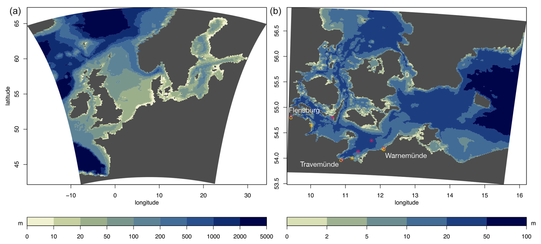
Figure 1 Bathymetry for the coarsest grid (a) and finest grid (b) of TRIM-NP. Marked are the locations of observed (orange) and modelled (red) water levels (circles) and wind data (asterisks).

2.2 Observational data

To evaluate the results of the numerical simulations for the three surge events in the western Baltic Sea, hourly water level data from the Travemünde, Warnemünde and Flensburg (Germany) gauges (orange circles in Fig. 1) provided by the Waterways and Shipping Administration, Germany (WSV, 2023), were used. In addition water levels from the Landsort (Sweden) gauge provided by the Swedish Meteorological and Hydrological Institute (SMHI, 2024) and from the Degerby (Finland) gauge provided by the Finish Meteorological Institute (FMI, 2024) were used. Water levels from Landsort and Degerby are frequently used as proxies for the total water volume of the Baltic Sea and to estimate prefilling (e.g. Janssen et al., 2001; Hupfer et al., 2003; Mudersbach and Jensen, 2009). To evaluate the quality of the wind fields driving the hydrodynamic hindcast, observational data (orange asterisks in Fig. 1) from the German Weather Service (DWD) for Boltenhagen near Travemünde, Warnemünde and Schönhagen were used (DWD, 2024). Schönhagen was used for comparisons near Flensburg as wind observations at Flensburg have data missing around the event maxima and are more influenced by land–sea interaction. As hindcast data were available hourly, only data at full hours were used for comparison for both the water level and wind, even if the observational data at higher frequencies were available. The simulated wind speed at each full hour represents the instantaneous value of the last model time step, which is adjusted to be comparable to the observational values, which are typically the mean of the last 10 min before the full hour.

2.3 Methods

2.3.1 Prefilling

Inflow and outflow processes across the Danish Straits with characteristic timescales of about half a month or longer change the volume of the water in the Baltic Sea (Weisse et al., 2021). Such volume changes are often referred to as prefilling or preconditioning and lead to an increase or decrease in water levels in the Baltic Sea (e.g. Mudersbach and Jensen, 2009; Lehmann and Post, 2015). As such volume changes can not directly be inferred from observations, proxies are normally used. A frequently used proxy is the water level from the Landsort (Sweden) gauge, which has shown to correlate well with Baltic Sea prefilling (e.g. Mudersbach and Jensen, 2009; Lehmann and Post, 2015). Additionally the time series of the gauge station at Degerby (Finland) has also been used as a proxy for the prefilling (e.g. Janssen et al., 2001; Bellinghausen et al., 2025).

In the present study a model simulation is available for the entire Baltic Sea basin so that the prefilling or the Baltic Sea volume anomaly (BSVA) can be estimated directly. It is derived by summing the water volume anomaly of each grid cell, which is defined as the product of the area represented by each grid cell and the corresponding water level anomaly. It is finally divided by the total area of the Baltic Sea to obtain the sea level anomaly caused by prefilling. As the prefilling of the Baltic Sea takes place over a longer period, days to weeks, a moving average over several days is usually used to describe the amount of the prefilling. Here we used a 7 d moving average, which is close to the 8 d averaging used in Soomere et al. (2015) for describing the amount of prefilling in the Baltic Sea.

2.3.2 Estimation of return periods

Several methods can be used to estimate return periods. Here, the generalized extreme value (GEV) method (Coles, 2001) based on annual maxima was applied to the 66 years of hindcast data. In order to calculate the GEV distribution, block maxima have to be derived over a certain time period. The definition of the time period depends on the variable. For wind and wind-related variables, such as extreme water levels, the storm season between autumn and spring (Eelsalu et al., 2014) or summer and the following summer (Liu et al., 2022) is often used. Especially for the Baltic Sea, possible prefilling at the end of the year can also influence extreme water levels in the following year, which would then cause dependent variables. Here, however, we have chosen the calendar year (January to December) to derive the block maxima. One reason is that the extreme event of interest occurred in October 2023, and as our dataset ends in 2023, we would not have the full storm season 2023–2024 and would be missing this event. A comparison with the results using block maxima from July to June shows only minor differences at the longer periods (not shown).

2.3.3 Effective wind

Wind statistics in the southwestern Baltic Sea show high frequencies of westerly components, especially for strong winds. However, strong westerly winds do not generate high water levels in the southwestern Baltic Sea, so using all wind directions without modification may lead to biased statistical measures of extreme water levels. We are, therefore, only interested in the strong winds that are responsible for the generation of extreme water levels, i.e. winds coming from a particular direction depending on the orientation of the coast. In order to calculate return values only for such wind components, the concept of the effective wind (Ganske et al., 2018) has been used. The effective wind is an orthogonal projection of the wind vector onto the pre-selected prevailing surge-generating wind direction. Thus, instead of using only wind events within a given directional range, each wind event with its orthogonal portion of wind speed relative to a defined direction is used for statistical analysis. Here, for simplicity, we used as a reference direction the wind direction that occurred during the highest water level event during the hindcast period at each of the three sites. Using this approach, the effective wind direction is northeast (42.6°) at Travemünde, north (354.6°) at Warnemünde and east (90.6°) at Flensburg. With these wind directions the effective wind is derived and used to estimate the return values for each location.

3 Results

3.1 Description of the three storm surge events

The three severe storm surge events in 2017, 2019 and 2023 affecting the German Baltic coast showed very high peak water levels, while the wind speed during the events varied from moderate (2017, 2019) to strong (2023). The wind directions also differed between the events. While the events in 2017 and 2019 were dominated by northerly winds, easterly winds were prevailing during the most recent event in 2023.

In 2017, before the onset of the event, a high-pressure system was located between the British Isles and Iceland (Lefebvre and Haeseler, 2017). As a consequence, the low-pressure system responsible for the storm surge event in the western Baltic Sea took a relatively northern track from the Norwegian Sea over Scandinavia and the Baltic Sea toward northeastern Europe. Over the Baltic Sea, associated wind fields initially came from westerly directions and changed towards more northerly and northeasterly directions over the southwestern Baltic Sea during the passage of the cyclone. During the event, the maximum wind speeds over the southwestern Baltic Sea were very moderate. They reached about 15 m s⁻¹ 6–12 h prior to the observed peak water levels and only about 10 m s⁻¹ at the times of surge maxima (Fig. 2). However, observed surge levels were high (with a maximum of 1.73 m at Travemünde, 1.58 m at Warnemünde and 1.76 m at Flensburg) and led to the event being a once-in-10–20-year event (Liu et al., 2022; https://stormsurge-monitor.eu, last access: 25 June 2025). In the hindcast, both modelled wind and water level fields agree well with observations. Here, maximum surge heights are 1.76 m at Travemünde, 1.66 m at Warnemünde and 1.76 m at Flensburg (Fig. 2).

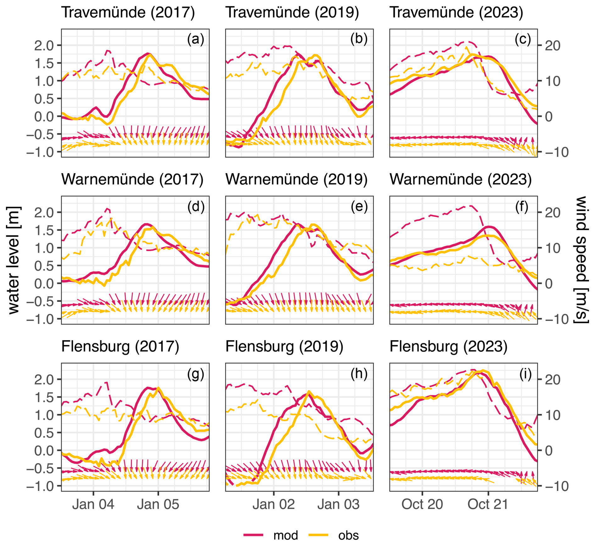
Figure 2 Time series of the water level (solid line), wind speed (dashed line) and wind direction (arrows) for observations (orange) and simulations (red) at Travemünde (a, b, c), Warnemünde (d, e, f) and Flensburg (g, h, i) for the storm surge in 2017 (a, d, g), in 2019 (b, e, h) and in 2023 (c, f, i).

During the 2019 event, the large-scale atmospheric circulation pattern was comparable to that for the event in 2017. Again, an atmospheric high occurred over the British Isles and the low-pressure system responsible for the storm surge event in the western Baltic Sea travelled along a track from northern Scandinavia, over Finland and towards the eastern Baltic states. The winds initially came from westerly directions and subsequently turned toward northerly directions at the times of the maximum water level in the southwestern Baltic Sea. Peak surge heights were comparable to those during the 2017 event and reached values of 1.72 m in Travemünde, 1.65 m in Warnemünde and 1.57 m in Flensburg (Fig. 2). While wind directions were comparable to the 2017 event, wind speeds were higher (Fig. 2). Again, hindcast wind and water levels agree well with observations, with modelled peak surge levels reaching 1.75 m in Travemünde, 1.66 m in Warnemünde and 1.57 m in Flensburg.

The most recent event on 20 October 2023 showed very different characteristics. Here the large-scale atmospheric circulation was characterized by a high-over-low weather pattern, that is, a blocking high-pressure system over Scandinavia and a relatively stable low-pressure system between the British Isles and west of France (DWD, 2023). In contrast to the other two events, this atmospheric situation lead to strong pressure gradients over the western Baltic Sea and correspondingly to strong easterly winds that have a high potential to strongly pile up water masses in the western Baltic Sea (Feistel et al., 2008). While the observed maximum water levels at Travemünde (1.75 m) and Warnemünde (1.46 m) were similar or even lower than those during the previous two events, in Flensburg, a very high value of 2.25 m was reached, substantially exceeding the maxima of the 2017 and 2019 events. The hindcast peak surge levels of 1.68 m in Travemünde, 1.59 m in Warnemünde and 2.19 m in Flensburg agree well with observations (Fig. 2). Wind speeds during the event were substantially higher than in 2017 and 2019, with the simulated wind speed exceeding 20 m s⁻¹ at all three locations. Hindcast and observed wind speeds agree well in Travemünde and Flensburg, while in Warnemünde the observed wind speed is considerably lower than in the hindcast. Note that this offset can be mostly explained by the fact that model grid points off the coast were used for comparison with observations on the coast as they were the only available ones in the area. The wind speeds off the coast are typically higher than over land. In addition, in 2023, as the dominant wind direction is from the east, the observational site is shadowed by the coast, which strongly enhanced the difference between land and open-sea winds.

The atmospheric situation during the 2023 event was comparable to that during the devastating 1872 flood event in the western Baltic Sea (Bork et al., 2022; Meyer et al., 2024). In contrast, the atmospheric situation during the 2017 and 2019 events was considerably different with prevailing moderate wind speeds from the north. In this case the fetch of the area of the wind influence was limited due to complicated topography of the Danish Straits, and it suggests that during these events factors other than the prevailing wind field contributed substantially to the observed peak water levels. To better understand the role of different processes and their contributions to the observed high water levels, the water level components associated with these processes were estimated and analysed separately and in the context of the total water level.

3.2 Main drivers contributing to the three storm surge events

3.2.1 Prefilling of the Baltic Sea

The estimated BSVA closely follows the modelled water levels at the grid cell closest to the Landsort location, apart from some high-frequency fluctuations (Fig. 3). Both time series are also comparable with the observations from the Landsort gauge (Fig. 3), although there are some discrepancies. In particular, for the 2023 event the observed water level at Landsort is about 0.15 m higher than that simulated at the time of the storm surge maximum. When using the time series of the gauge station at Degerby (Finland) the water level is again relatively close to the simulated BSVA (Fig. A1). Since we can determine the BSVA and thus the prefilling effect directly from the model data, the BSVA is used instead of the Landsort water levels for a consistent model-based analysis.

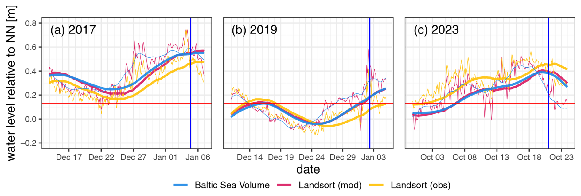
Figure 3 Hourly (thin lines) and 7 d average (thick lines) time series of the Baltic Sea volume (blue), simulated water level at Landsort (red) and observed water level at Landsort (orange) before and around the time of the surge maximum (vertical blue lines) for the event in 2017 (a), in 2019 (b) and in 2023 (c). The horizontal red line represents the long-term mean volume of the Baltic Sea. NN: Normalnull.

In order to quantify the contribution of the prefilling to the total water level during the storms, the BSVA was additionally averaged over 7 d (thick lines in Fig. 3) so that the index represents the deviation from the mean state 1 week prior to the water level event maximum. This appears to be a more relevant index than an instantaneous BSVA, as the latter is artificially uniform over the entire basin, whereas in reality the access of water is redistributed unevenly across the basin. This can be seen for the example of the storm of 2023, where the instantaneous BSVA is about 0.18 m lower than the 7 d average. In this case there is an outflow of the water through the Danish Straits, starting already several days before the storm maximum, which diminishes overall instantaneous BSVA. At the same time the rest of the prefilling is accumulated in the western Baltic Sea due to e.g. not only easterly winds but also the water swinging back in seiche-like oscillations. Finally, the long-term mean Baltic Sea volume anomaly (0.13 m) was subtracted from the 7 d average to derive the BSVA contribution to the water level maximum. Thus, during the 2017 event, prefilling contributed about 0.41 m, which constitutes about 24 % of the peak water level in Travemünde, 25 % in Warnemünde and 23 % in Flensburg. During the 2019 event, the contribution from prefilling was negligible at about 0.05 m and accounted for only about 3 % of the total peak water levels at all locations. For the 2023 event, the prefilling was about 0.25 m above average, thus contributing about 12 % of the peak water level in Flensburg, 15 % in Travemünde and 16 % in Warnemünde.

3.2.2 Wind

Strong onshore winds pushing the water towards the coasts are usually the main driver of storm surges (Pugh and Woodworth, 2014). To disentangle the contribution of the local wind fields to the peak surge levels at the three events, a set of model sensitivity experiments was carried out. For the three events, the TRIM-NP model was restarted from average (climatological) conditions 60, 48, 36, 30 and 24 h prior to the timing of the peak surge levels in each event. In all experiments, the original atmospheric forcing from the multidecadal hindcast was used. This allowed for an estimate of the contribution of the local wind fields to the observed peak water levels. The results are summarized in Fig. 4, and each event is represented by one location for which the original storm surge was most prominent. For the event in 2017 the maximum surge levels caused by the short-term winds of different durations reached 1.41 m when the area was exposed to the wind influence for 60 h (Fig. 4). This is 0.35 m lower than the maximum water level obtained from the full model simulation. The underestimation holds for both before and after the storm and corresponds well with the magnitude of the estimated Baltic Sea prefilling observed and simulated for this event (Fig. 3). In this case the wind influence could explain about 80 % of the water level elevation during the storm, while the other 20 % is attributable to prefilling and non-linear interactions. The example of Travemünde is representative of other locations as well (not shown). Thus, according to the sensitivity experiments, 77 %–86 % of the maximum water level in Flensburg can be attributed to the local wind influence. The total water level in Warnemünde was lower during the storm event in 2017, which is reflected in a somewhat smaller contribution from the local wind and larger contribution from other processes (approx. 70 % to 30 %).

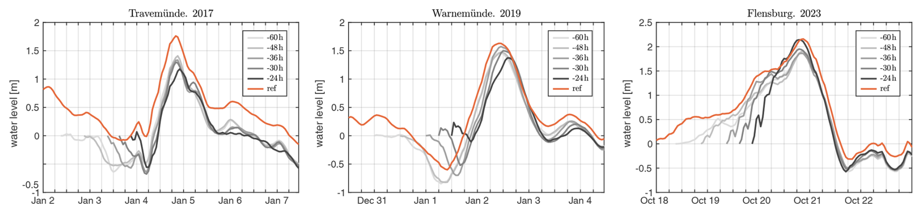
Figure 4 Water levels generated by short-term winds (starting 24 to 60 h prior to the storm maxima, grey lines) without consideration of previous conditions. Water level time series for the three storms at the locations of the storm's maximum impact from the reference simulation (red).

The event in January 2019 showed similar behaviour, but the differences between the maximum water level from the full simulation and the short-term wind simulations were between 0.07 and 0.16 m. This is also in accordance with the small prefilling rates of several centimetres (Fig. 3) for this event. In summary, the peak water levels in 2017 and 2019 were similar (Fig. 2); the prefilling was lower in 2019; and the influence of the wind was slightly higher, consistent with slightly higher wind speeds in 2019. The combination of both effects explains the total water levels well. This shows that different combinations of the two main forcing factors can lead to similar extreme water levels. Moreover, even very similar atmospheric conditions may lead to different relative weighting of the contributions of these factors and to different resulting water levels. The event in 2023 occurred under different atmospheric conditions, namely long-lasting easterly winds, which alone could cause up to 1.9 m surge levels at Flensburg with wind influence starting 60 h prior to the water level maximum. Unlike previous examples, the model results for 2023 show higher water levels with less wind influence (dark-grey vs. light-grey lines in Fig. 4). This can be partly explained by the fact that the same wind influence causes higher surge when the affected area has smaller total water depths. For example, at the time when the “−24 h” experiment starts at zero surge levels (21:00 UTC, 19 October), the surge height has already reached 1.3 m in the “−60 h” experiment. As a consequence, the same wind at this time affected 1.3 m deeper water in the −60 h simulation, which could account for the reduction of about 5 %–10 % in peak surge heights. Consequently, the subsequent water elevation in the −60 h simulation was lower than in the −24 h simulation when both were exposed to the same wind influence. Given that the positive water elevation 60 h prior to the water level maximum is more realistic for this event, it is argued that the maximum wind-related contribution can be better represented by the −60 h simulation. It demonstrates that there is an underestimation of the maximum water level by 0.25 m when only wind conditions are considered compared to the full simulation. This is in fairly good agreement with the prefilling calculated for the event, leaving the direct wind influence responsible for 85 %–90 % of the total maximum water levels. For the other locations, Travemünde and Warnemünde, the maximum total water levels during the event were considerably lower than in Flensburg, but still the sensitivity experiments showed that water levels were about 0.25 m lower when only the local wind effect was considered. This is in line with the magnitude of the prefilling common for the entire region. Consequently, the relative contribution from the wind-driven water levels decreases to 80 %–83 % for these locations.

3.2.3 Other processes

In addition to the effects mentioned above, water levels in the Baltic Sea are influenced by the atmospheric pressure and can experience variations in the decimetre range due to the inverse barometer effect (e.g. Leppäranta and Myrberg, 2009). However, this process is related to the immediate atmospheric conditions and is directly considered by the hydrodynamic model. Thus, in the remainder of this study the water levels referred to as wind-related do technically include the inverse barometer effect.

The Baltic Sea is a micro-tidal environment, and tides can contribute 0.05–0.2 m to the water level elevation in the southwestern Baltic Sea, depending on the location (e.g. Medvedev et al., 2016). A tide-only simulation was used to estimate the tidal signal during the event maximum. According to the simulations, the tidal component during the peak water level reached about 0.03 m in 2017 for Travemünde, −0.07 m in 2019 for Warnemünde and 0.1 m in 2023 for Flensburg. Although it is relevant to include the tidal signal in the simulations to account for both the tidal elevation and tide–surge interactions, especially when single events are reconstructed and compared with observations, the tides can be neglected in the long-term analyses of extremes (e.g. Gräwe and Burchard, 2012). Therefore, in the present study, tides are not analysed explicitly but are kept in the residual part of the water levels.

Another process that can contribute to the total water level variations is related to seiches. Seiches are standing waves that oscillate freely in semi-enclosed basins under the influence of atmospheric forcing and persist even after the winds have ceased or even just started to decay. In the Baltic Sea and its bays various modes of seiches with different periods have been observed or discussed (e.g. Leppäranta and Myrberg, 2009). Although the phenomenon has been known and investigated for a long time, there are still controversial aspects about the main periods of the oscillation and whether there are basin-wide or rather combinations of local bay oscillations (e.g. Jönsson et al., 2008; Weisse et al., 2021). This makes the clear separation of the seiche component rather uncertain, especially in the long-term perspective. This process is taken into account in the model simulations but is not investigated here separately from a climatological point of view.

An additional process that contributes to the overall water level in coastal regions is the wave set-up. As the waves break in the surf zone, the momentum associated with the wave is transferred to the water column, causing an increase in water level towards the coast. Depending on the wind and wave situation during an extreme storm event and the coastal location, the wave set-up can contribute up to 30 % of the total water level on the Baltic Sea (Eelsalu et al., 2014) or up to 35 % on the Australian coast (Hetzel et al., 2024). Su et al. (2024) estimated the wave-induced set-up along the Danish coast and found that for the 2017 event the contribution along the western Baltic Sea was rather small with only 5 cm, which corresponds to less than 5 % of the total water level. For the 2019 and 2023 events, the contribution of the wave set-up could be larger as the wind speed and wave height were higher compared to 2017. However, in order to estimate the contribution to the total water level, knowledge of the bed slope along the coastline and sufficiently resolved wave information is required. As both types of information are not available, the contribution of the wave set-up to the total water level was not addressed.

3.3 Climate perspective

The three events discussed had surges that ranked among the highest observed on the German Baltic Sea coast since the early 1950s. Furthermore, the events themselves occurred in close proximity over the past 7 years. This raises questions about the extent to which these events were unusual, whether and how the frequency or severity of such events has changed over time, and how contributing factors such as prefilling or prevailing wind conditions may have changed. In the following, these questions are addressed using insights from the multidecadal hindcast.

3.3.1 How unusual were the events?

To place individual events in a historical context, their return periods, using the GEV method, are estimated. The return values derived provide an indication of whether the events fall within the expected range of extreme events or may be at the upper boundary (Fig. 5). The estimated return values for the total water level show that the 2017 event at Travemünde is one of the highest in the simulation period with a return period of about 30 to 40 years. The 2019 event has a similar return period, and the water level of 2023 still has a return period of 10 to 20 years. At Warnemünde, the 2019 event has a higher return period of more than 50 years, followed by the 2017 event with a similar return period, and the 2023 event still has a return period of almost 20 years. The analysis of the total water level at Flensburg shows that the 2023 event is an exceptional event in the simulation period with a return period of 66 years. Note that the 66-year return period is the upper limit due to the length of the simulation period. Given the estimated return curve and the wider confidence interval, the water level would easily exceed the 100-year period. For Flensburg, the 2017 event is also one of the highest, with a return period of almost 20 years; only the 2019 event, even if it falls into the category of severe storm surges, is a fairly normal event with a return period of about 4 to 5 years. It should be noted that the derived return value curves from the simulations differ from those estimated from observations (e.g. in Liu et al., 2022; https://stormsurge-monitor.eu, last access: 25 June 2025). This may be due to the longer observation period than the modelling period. For example the prominent southwestern Baltic Sea extreme event of 4 January 1954 is absent in the hindcast data. Another reason for discrepancies could be a slightly inaccurate representation of some event maxima by the simulation or the absence of absolute event maxima by the simulation if they occurred between full hours and are therefore not included in the hindcast time series. Such a discrepancy between the return value estimated from observations and from simulations is also found and discussed in detail by other authors (e.g. Soomere et al., 2018).

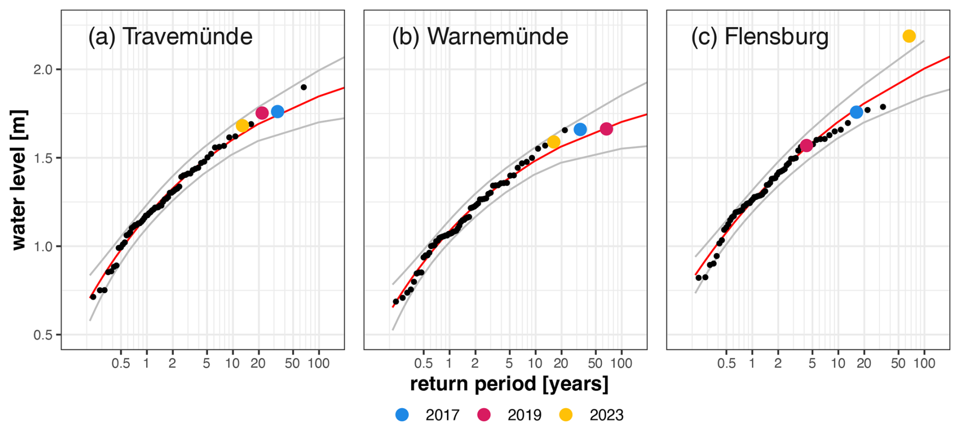
Figure 5 Return values (red curve) using GEV estimated from simulated annual maximum water levels (black dots) at Travemünde (a), Warnemünde (b) and Flensburg (c). Grey lines indicate the 95 % confidence interval of the return values. Maximum water levels of the recent events are represented by coloured dots (2017: blue; 2019: red; 2023: orange).

However, the question remains as to whether the contributing factors were also exceptional and for which events which contributions were more crucial. In order to investigate this, the return value of the annual maximum of the BSVA (7 d average) was analysed as an indicator of prefilling (Fig. 6). None of the BSVAs during the three events show an exceptionally high return period. The BSVA for the 2017 event has a typical return period of 1 to 2 years. For the other two events (2019 and 2023), the BSVAs are still above the average BSVA. However, the return periods only range from weeks to months. This suggests that, under different circumstances and in combination with more extreme BSVA conditions, the total water levels could have been higher for these three events.

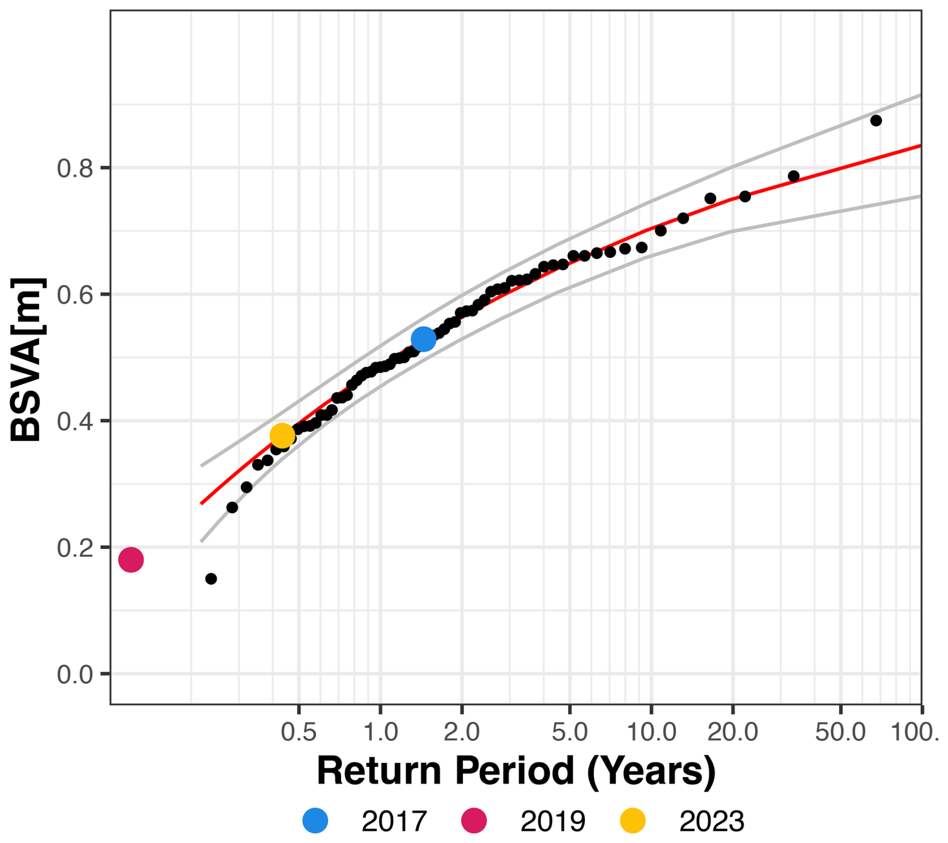
Figure 6 Return values (red curve) estimated with GEV from the simulated annual maxima of the BSVA 7 d average (black dots). Grey lines indicate the 95 % confidence interval of the return values. Average BSVA values within 7 d prior to the maximum total water levels of the recent events are represented by coloured dots (2017: blue; 2019: red; 2023: orange).

The extent to which the wind conditions were unusual during the three events was analysed using effective wind speeds (Fig. 7). For Travemünde the effective wind associated with the 2017 event can be expected on average once every 1–2 years. The return periods for the effective wind during the two events in 2019 and 2023 are still moderate, about 4 and 7 years respectively. For Warnemünde the two events of 2017 and 2019 were highly unusual in terms of effective winds. Here such events could be expected once in 20 to 30 years. For Flensburg, the event in 2023 is outstanding also in terms of the effective wind. Here a return period of 66 years was estimated, which shows that the 2023 event in Flensburg was exceptional, with the wind being the major contributing factor.

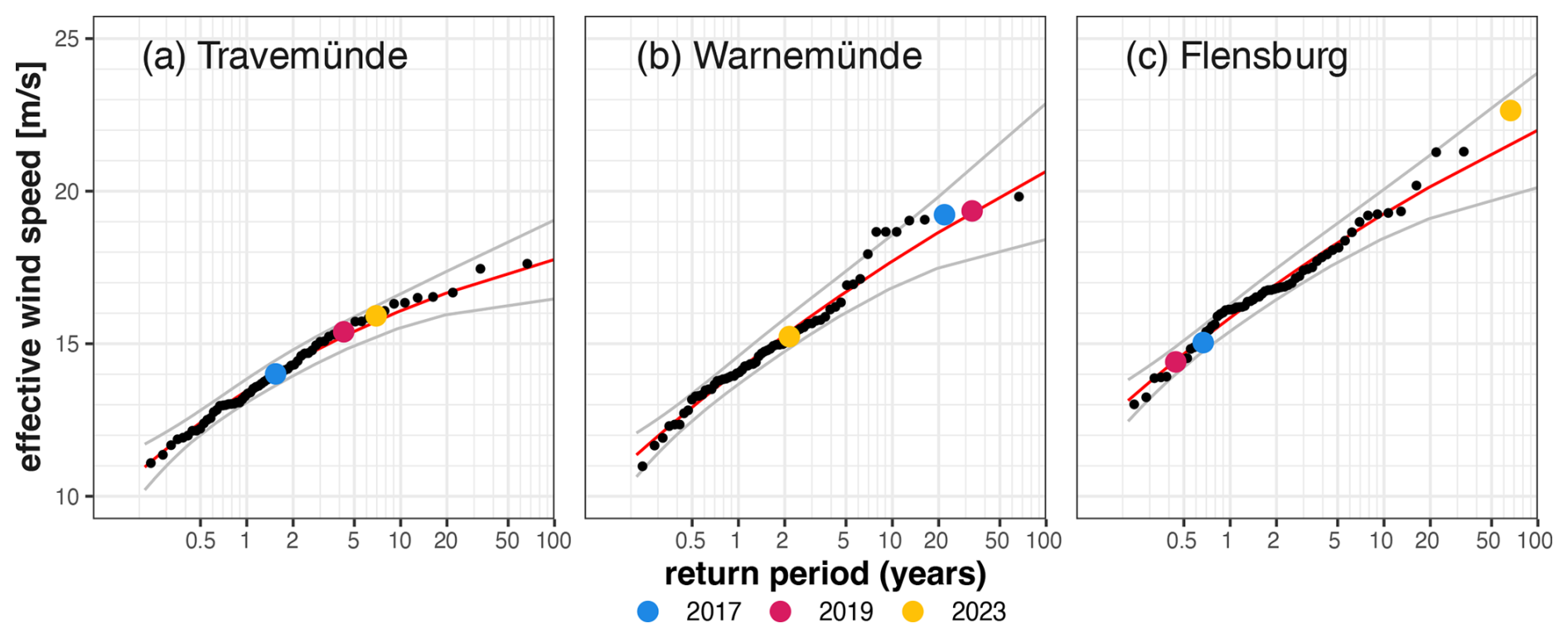
Figure 7 Return values (red curve) using GEV estimated from the simulated annual maximum effective wind speed (black dots) for Travemünde at Lübecker Bight (a), for Warnemünde at Mecklenburger Bight (b) and for Flensburg at Flensburger Fjord (c). The grey lines indicate the 95 % confidence interval of the return values. Recent maximum effective wind speeds are represented by coloured dots (2017: blue; 2019: red; 2023: orange).

While for the 2019 event, wind speed and direction seem to be the main reason for the extreme high water levels, for the other events, neither BSVA nor wind speed alone is a reasonable explanation for such extreme water levels. A further analysis of the joint distribution of the event maximum water level and its two main contributors, BSVA and wind speed, could indicate the special nature of these events. Further analysis of three different periods will reveal whether the contribution of each factor has changed over time. Only water level events exceeding 1 m are used in the following.

The joint distribution of the maximum water levels during each extreme event and the BSVA averaged over the 7 d prior to the event maximum is shown as a scatterplot for different locations (Fig. 8). For Travemünde there are events with a higher BSVA than during the three events 2017, 2019 and 2023. None of these events has a total sea level exceeding the maxima of the three most recent events. There is, however, one event with a BSVA below average that has a higher total water level. The event happened on 13 January 1987 and was characterized by strong winds (up to 25 m s⁻¹) from the northeast, which corresponds to the prevailing wind sector for generating maximum surge in Travemünde. This example indicates both the sensitivity of the surge height to the exact local wind directions and a possibility for much higher surge magnitude in the case that such wind conditions coincide with the larger BSVA. Warnemünde shows a similar distribution of water levels and BSVA during extreme events. Notably, the 1987 event resulted in a much lower water level here than in Travemünde, as the wind direction was not optimal for generating extreme surge in Warnemünde. At Flensburg, the 2023 event again shows its peculiarity with an extreme water level which has never occurred in the simulation period and a moderate BSVA. The 2017 event is characterized by the relatively high BSVA, and the 2019 event is not remarkable compared to other extreme events. When comparing different periods, there is no clear tendency towards more or less BSVA contribution to the extreme water levels. There is almost a slight decrease in the contribution of BSVA in the most recent period compared to the previous 20 years, with the eight highest BSVAs having occurred the during 1980–2001 period.

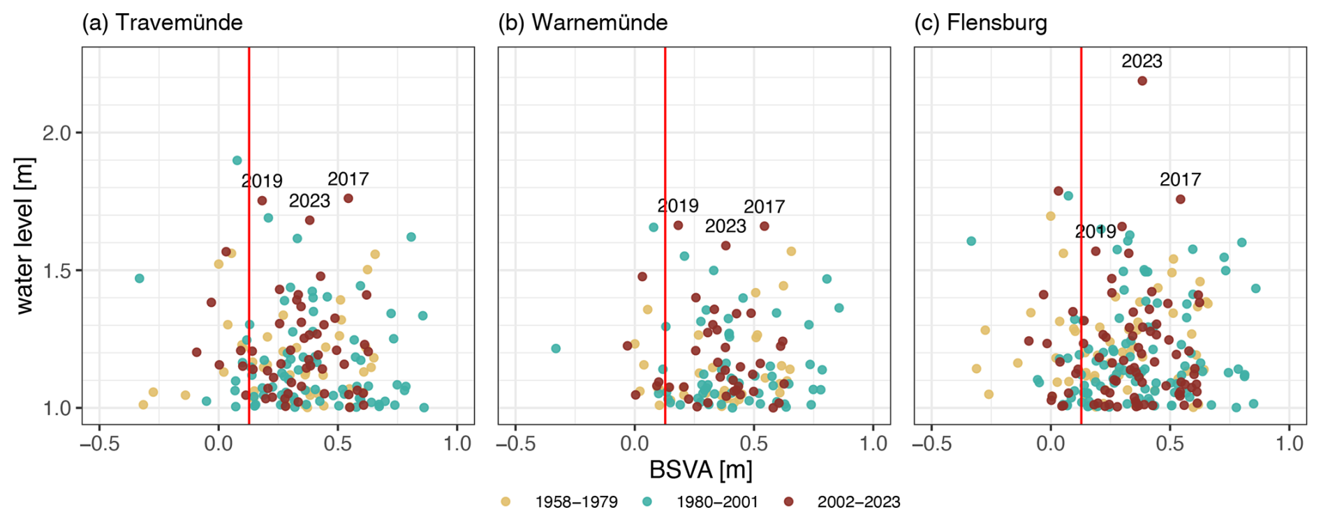
Figure 8 Scatterplot of the water level and BSVA averaged over the 7 d prior to the event maximum at Travemünde (a), Warnemünde (b) and Flensburg (c). Coloured dots indicate events from three 22-year-long periods; the events discussed are annotated with their years. The vertical red line indicates the long-term mean BSVA.

As the surge is generated over a period of time, not only the wind conditions at the time of the surge but also the winds for at least several hours prior to the surge are important. Thus, the joint distribution of the total water level maximum and the wind speed and direction averaged over the 6 h prior to the water level maximum was analysed (Fig. 9). The wind speed during the 2017 event was on the rather lower side of the distribution compared to all other extreme water level events (above 1.5 m). Compared to all severe storm surge events above 1.5 m, the 2017 event had the lowest wind speed at Travemünde and Warnemünde but with a rather optimal mean wind direction heading from north northeast towards the coast. Even at Flensburg, where there are some severe storm surge events with lower wind speeds, the wind speed in January 2017 was low compared to events with similar water levels. During the 2019 event, the wind speed at Travemünde was one of the highest during an extreme water level event, and while it was high for Warnemünde and Flensburg, it was not exceptional compared to other events. Both events show a northerly component, which tends to lead to high water levels at Travemünde and Warnemünde. The 6 h mean wind before the 2023 event for Travemünde and Warnemünde was high but comparable to other events with a high water level. There was one event (13 March 1969) with the 6 h averaged wind speed and direction comparable to those of the 2023 event for Flensburg. However, the resulting water levels were significantly lower, partly because the BSVA was slightly negative during the event in 1969 and partly because of lower peak wind speeds immediately before the event maxima.

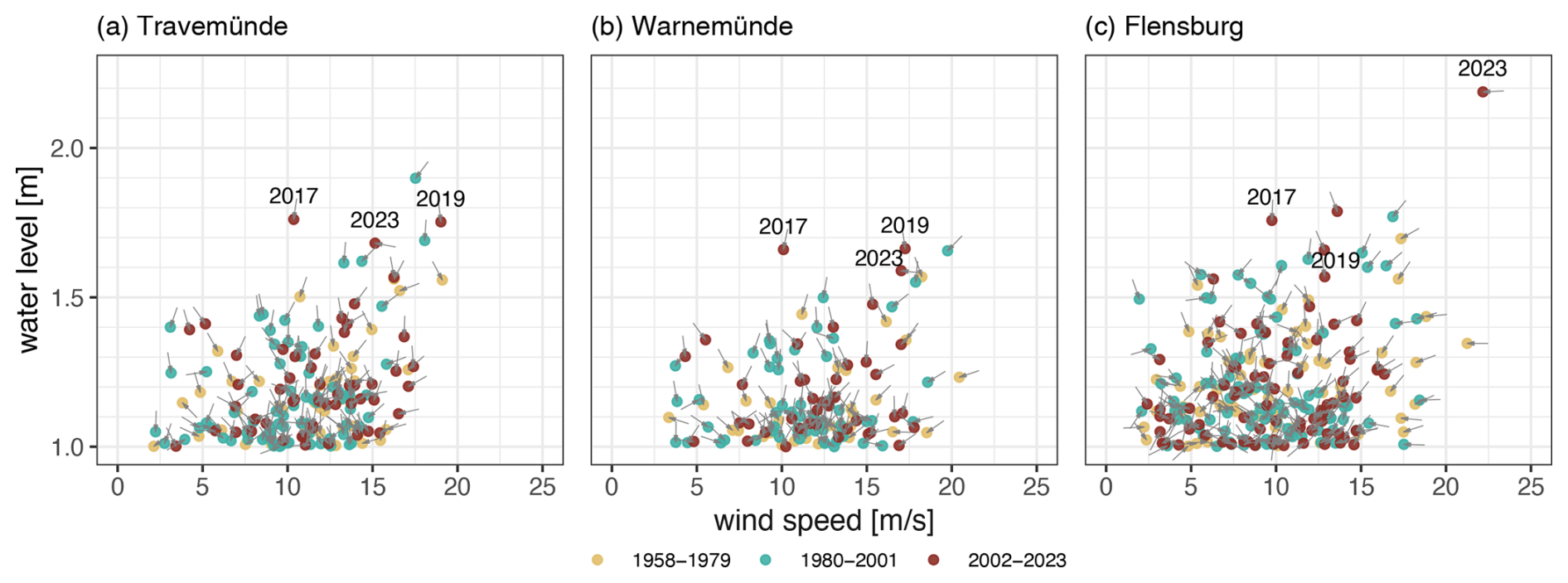
Figure 9 Scatterplot of the water level maximum and wind speed averaged over the 6 h before the event maximum at Travemünde (a), Warnemünde (b) and Flensburg (c). Coloured dots indicate three different 22-year periods; the events discussed are annotated with their years. Arrows indicate the average wind directions 6 h before each event.

There is no clear trend in the temporal variability in the joint occurrence of wind conditions and water level. While Travemünde shows a slight increase in the number of events with wind speeds above 15 m s⁻¹, these higher wind speeds do not necessarily lead to an increase in the number of water level events above 1.5 m. At Warnemünde, events with even higher wind speeds than during the recent three events occurred in earlier periods. At Flensburg, with the exception of the 2023 event, wind speeds above 17 m s⁻¹ occurred only in periods before the most recent one.

3.3.2 Long-term changes in the storm surge climate

To better investigate possible temporal variability and long-term trends of extreme water level events, time series of hourly hindcast water levels from 1958–2023 were analysed (Fig. 10). The time series show pronounced short-term variability at all three locations that may mask potential long-term changes. For the analysis of the variability in extremes, the storm surge classification used by the German Federal Maritime and Hydrographic Agency (Bundesamt für Seeschifffahrt und Hydrography, BSH) was applied. The BSH uses the following thresholds to classify storm surges in the Baltic Sea:

• 1.

  storm surge – an event with a peak water level between 1 and 1.25 m above the mean water level (MWL)

• 2.

  medium storm surge – an event with a peak water level between 1.25 and 1.5 m above MWL

• 3.

  severe storm surge – an event with a peak water level between 1.5 and 2 m above MWL

• 4.

  very severe storm surge – an event whose peak water level exceeds 2 m above MWL.

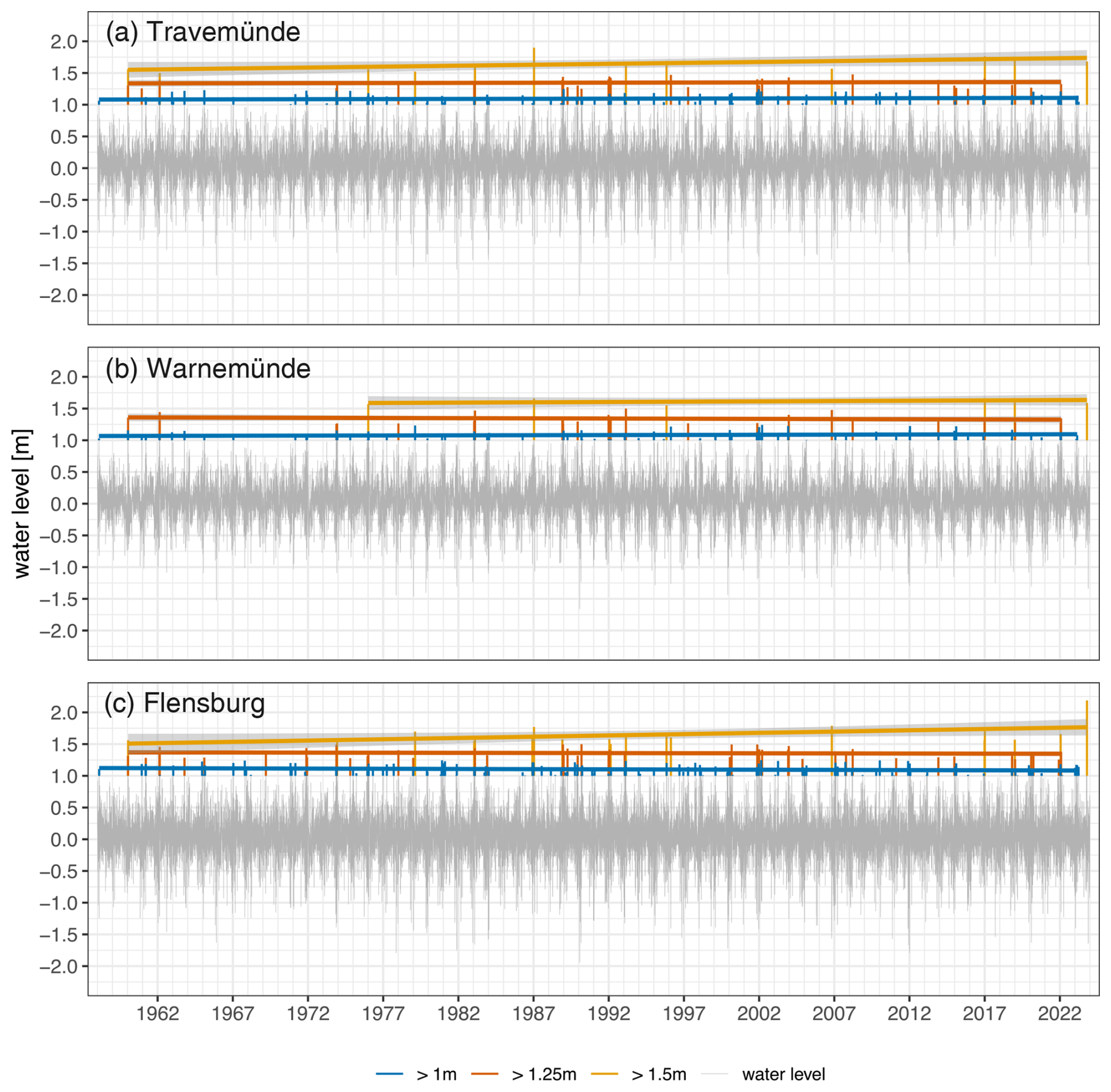
Figure 10 Simulated time series of hourly water levels for the period 1958 to 2023 at Travemünde (a), Warnemünde (b) and Flensburg (c). Storm surge events between 1 and 1.25 m are marked in blue, medium surge events between 1.25 and 1.5 m are in red, and severe surge events exceeding 1.5 m are in orange. Coloured lines represent linear trends calculated for the respective type of events with the 95 % confidence interval.

As only the 2023 event exceeds the threshold for a very severe storm surge, only the other three categories are used in the analysis and the 2023 event is treated as a severe storm surge.

The storm surge classification was superimposed onto the hourly water level time series (Fig. 10). The sequences of storm surges in the different intensity classes show periods with lower and higher values. For example, lower values occurred in the late 1960s and early 1970s, while surges became more frequent from the late 1980s to mid-1990s.

The time series further reveals that the three events of 2017, 2019 and 2023 were among the highest in the simulation period. For Flensburg the event in 2023 was the largest during the hindcast period starting in 1958. This cluster of three events in the last 7 years indicates an increase in the number of events above 1.5 m above MWL, but this positive trend is subject to great uncertainty. Furthermore, for the two lower categories, storm surge (1) and medium storm surge (2), there is no long-term trend for all three locations. Similar analysis of the time series of the BSVA and the wind speed shows high short-term variability and small linear trends that are accompanied by large conference intervals (see Figs. B1 and B2 in Appendix B).

4 Conclusions

Three recent extreme storm surge events in the southwestern Baltic Sea were analysed and put into a climate perspective. The comparison of water levels at three locations along the German Baltic Sea coast generally showed good agreement between the hindcast model simulations and observations. Both datasets confirm that the three events were among the highest on the German Baltic Sea coast, at least within the period from 1958–2023. We further focused on the relative contributions of the two key factors associated with storm surges in the Baltic Sea, namely the prefilling caused by the inflow of water masses from the North Sea during days to weeks prior to the event and a component induced by the short-term wind influence during the storm.

The events in 2017 and 2019 can be associated with high pressure located over western Europe (British Isles, France) which led to a storm track across Scandinavia and towards eastern parts of Europe, resulting in northerly winds in the southwestern part of the Baltic Sea. During the 2017 event, the wind speed was relatively moderate, but the Baltic Sea volume was relatively high, constituting about 25 % of the total maximum water level. The 2019 event showed high wind speed, and, especially in Warnemünde, the wind direction (from the north) was rather favourable for creating high water levels on the coast. The contribution of prefilling was small, in the order of 3 %, during the 2019 event. The 2023 event was dominated by extremely high wind speeds caused by a Scandinavian blocking situation. High pressure over Scandinavia and the low-pressure system between France and the British Isles led to prevailing easterly winds over the western Baltic Sea, resulting in the highest water levels in the simulation period at one location (Flensburg). This is also confirmed by observations, and in the case of the 2023 event, the water level was the highest observed in the last 100 years (Kiesel et al., 2024). The prefilling during this event was moderate, but it still contributed 10 %–15 % of the total maximum water level depending on the location.

Additionally, both contributing factors were analysed in the context of historical storm events based on the model simulations for the past 6 decades. It can be stated that for the 2017 and 2019 events, the wind speed was not the highest during the storm event, especially when compared to other events with high water levels. Again, the 2017 event is relatively unique as the wind speed shortly before and during the event was only about 10 m s⁻¹ and thus lower than for all other events, with surge heights above 1.5 m within a 66-year period and wind speeds near Travemünde varying between 12.5 and 18 m s⁻¹. In contrast, the event of 2023 showed extreme water levels and extreme wind speeds unprecedented within at least the considered 66 years.

The analysis of the effective wind based on the wind directions favourable for the generation of high water levels at specific locations showed that the return periods for the 2017 and 2019 events at Warnemünde and the 2023 event at Flensburg were high – from 20 to at least 66 years. The same storm events caused much smaller effective winds for other locations, with the return values corresponding to a 1–7-year return period. This is reflected in the water level magnitudes on different parts of the coast and underlines the importance of accurate wind direction representation, which is particularly important for predicting extreme water levels. It can be further concluded that while the total water levels of the recent events are among the highest in recent decades, with a return period of 10 to 66 years, the Baltic Sea volume magnitudes were rather normal, with a return period of 1.5 years or less. It should be noted that calculating and estimating return values based on a limited sample size, such as 66 years, has limitations. This is particularly true for extreme events at the edge of the sample size, as the results may be uncertain and have a wide confidence interval. This suggests that longer return periods are possible, especially when compared to return periods estimated from observations (e.g. Liu et al., 2022; Kiesel et al., 2024).

The multidecadal analysis of the water level maxima exceeding 1 m showed that there is no clear trend in the evolution of extremes within the past 6 decades and that the interannual variability in extreme water level events in the southwestern Baltic Sea is rather high. This is in line with the findings of Feser et al. (2015) and Lorenz and Gräwe (2023), who discuss the variability in extremes and unclear trends when considering different historical periods. The same holds for the contributing components of the extreme water levels, where we found no increase in the frequency or magnitude of BSVA in recent decades but rather a small decrease in the last 20 years. No significant changes were observed for wind either (Bierstedt et al., 2015). Considering the non-exceptional nature of the contributing components during the recent events (with the exception of the wind conditions for Flensburg in 2023), it is probable that a combination of higher individual contributions can co-occur, potentially leading to higher total water levels under the present-day conditions, in line with the previous conclusions by e.g. Andrée et al. (2023).

Finally, it should be noted that the exception to these events was the combination and simultaneous occurrence of their individual contributions. Especially since some of these events could have had a higher water level with a different co-occurrence of high BSVA and high wind speed with favourable wind direction, analysing compound events is important.

Appendix A: Prefilling of the Baltic Sea

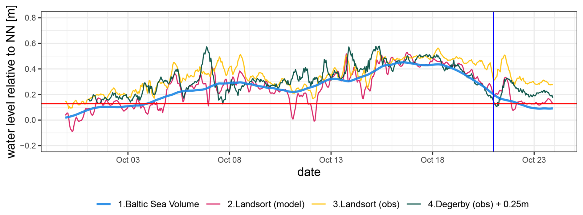
Figure A1 Time series of the Baltic Sea volume (blue), simulated water level at Landsort (red), observed water level at Landsort (orange) and observed water level at Degerby (green) before and around the time of the surge maximum (vertical blue lines) for the event in 2023. The horizontal red line represents the long-term mean volume of the Baltic Sea.

Appendix B: Long-term changes in the storm surge climate

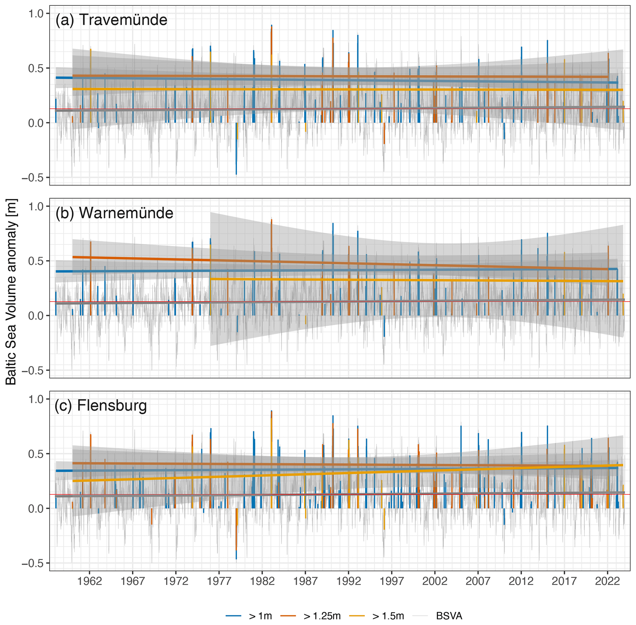
Figure B1 Simulated time series (grey) of the hourly Baltic Sea volume anomaly (BSVA) for the period 1958 to 2023 at Travemünde (a), Warnemünde (b) and Flensburg (c). For BSVA, storm surge events between 1 and 1.25 m are marked in blue, medium surge events between 1.25 and 1.5 m are in red, and severe surge events exceeding 1.5 m is in orange. The grey line represents the linear trend for hourly BSVA, and the coloured lines represent the linear trends calculated for each type of event with the 95 % confidence interval.

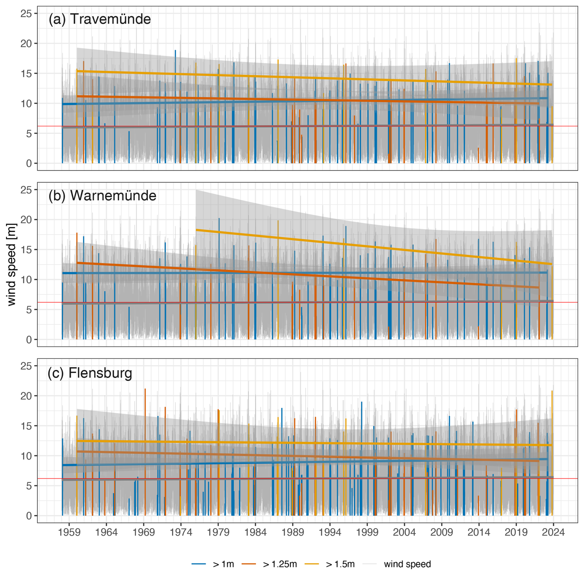
Figure B2 Simulated time series (grey) of hourly wind speeds for the period 1958 to 2023 at the offshore site for Travemünde (a), Warnemünde (b) and Flensburg (c). For wind speed, storm surge events between 1 and 1.25 m are marked in blue, medium surge events between 1.25 and 1.5 m are in red, and severe surge events exceeding 1.5 m are in orange. The grey line represents the linear trend for hourly wind speed, and the coloured lines represent the linear trends calculated for each type of event with the 95 % confidence interval.