It could have been much worse: spatial counterfactuals of the July 2021 flood in the Ahr Valley, Germany

After a flood disaster, the question often arises: what could have happened if the event had gone differently? For example, what would be the effects of a flood if the path of a pressure system and the precipitation field had taken a different trajectory? In this paper, we use alternative scenarios of precipitation footprints shifted in space, the so-called “spatial counterfactuals” to generate plausible but unprecedented events. We explore the spatial counterfactuals of the deadly July 2021 flood in the Ahr Valley, Germany. We drive the mesoscale Hydrologic Model (mHM) of the Ahr catchment with precipitation fields of this event systematically shifted in space. The resulting discharge is used as a boundary condition for the high-resolution two-dimensional hydrodynamic model RIM2D calibrated and validated for this area. We simulate changes in peak flows, hydrograph volumes, and maximum inundation extents and depths, as well as affected assets, and compare them to the simulations of the actual event. We show that even a slight shift in the precipitation field by 15–25 km eastward, which does not seem implausible due to orographic conditions, causes an increase in peak flows at gauge Altenahr of about 32 % and of up to 160 % at the individual tributaries. Also, significantly larger flood volumes of more than 25 % can be expected due to this precipitation shift. This results in significantly larger inundation extents and maximum depths at a number of analysed focus areas. For example, in the focus area around Altenahr, the increase in mean and maximum depths of up to 1.25 and 1.75 m, respectively, is simulated. The presented results should encourage flood risk managers as well as the general public to meet precautionary measures for extreme and unprecedented events.

1 Introduction

On 14–15 July 2021, an exceptional flood event struck a vast region in western Germany, Belgium, Luxembourg, and the Netherlands, causing more than 230 deaths and total economic loss of up to EUR 50 billion (Szönyi et al., 2022). In Germany alone, more than 180 people lost their lives, and loss estimates range between EUR 35 billion and 40 billion. The Ahr river valley in the Eifel mountains was a hotspot of flood impact with 134 deaths and two people still missing (DKKV, 2022). This is the highest human life loss due to a flood catastrophe in Germany since the storm surge in 1962 in northern Germany.

In the first half of July 2021, a low-pressure system formed over the North German Plain, resulting in a southwestward air flow strongly enriched with moisture from the Baltic Sea and the North Sea (Mohr et al., 2023). As a result, precipitation sums of up to 150 mm were recorded within 15 to 18 h in parts of the Ahr catchment. Using the hourly radar-based RADOLAN data (Weigl and Winterrath, 2009; Winterrath et al., 2018) and the daily station-based HYRAS dataset (Rauthe et al., 2013), Mohr et al. (2023) estimated the return period of precipitation to be of the order of 500 years in parts of the Ahr catchment. Kreienkamp et al. (2021) and Tradowsky et al. (2023) estimated a return period of about 400 years for daily precipitation sums in the period from April to September by pooling the HYRAS data over a larger region between the North Sea and the Alps. This heavy and intense rainfall resulted in an extreme catchment response, with strong field evidence for massive overland flow, where ephemeral drainages in forests and grassland turned into concentrated streams (Dietze et al., 2022). The rapid water rise within a few hours led to unprecedented water levels of up to 10 m, exceeding the instrumental record since 1947 and the historical high-water marks since 1804. Gauges Altenahr and Müsch (Fig. 1) were destroyed, so no discharge could be recorded instrumentally. The post-event peak flow reconstructions at gauge Altenahr range from 750 to 1100 m³ s⁻¹. Roggenkamp and Herget (2022) suggested a peak flow of 1000 m³ s⁻¹ or higher based on the recorded wrack marks, surveyed topography, and the application of Manning's equation with typical roughness values. The model-based flow reconstruction by Berkler et al. (2022) resulted in somewhat lower values between 750 and 1000 m³ s⁻¹, partly considering the backwater effect due to clogging of several bridges. The reconstructed peak flow exceeded the highest instrumental record of 236 m³ s⁻¹ in 2016 by three to more than four times. It reached about the same level as the reconstructed peak flow of the 1804 summer flood, for which a few historical high-water marks are available (Roggenkamp and Herget, 2014). Remarkably, the water levels during the 2021 flood exceeded those of 1804 by more than 2 m (Mohr et al., 2023), probably due to the aforementioned bridge clogging and resulting backwater effects but also due to denser settlements and higher macroscopic roughness at the present time. Considering the historical floods of 1804, 1888, 1910, 1918, and 1920 as well as recent instrumental records, Vorogushyn et al. (2022) estimated the local return period at gauge Altenahr to be more than 8500 years based on the peak flow reconstruction by Roggenkamp and Herget (2022). Due to limited records, the very high skewness of the time series, and the poor fit of the statistical model to the extremes, the return period estimates are associated with very high uncertainties.

The likelihood and intensity of extreme floods as in July 2021 can increase in a warmer climate due to increased heavy precipitation. Deploying ensembles of regional and global climate models, the extreme event attribution studies of Kreienkamp et al. (2021) and Tradowsky et al. (2023) suggested an increased likelihood of the observed maximum 1 d precipitation to occur in the present climate compared to the pre-industrial state (1.2 °C cooler) by a factor of 1.2–9. A further increase in the likelihood by a factor of 1.2–1.4 is suggested in a 2 °C warmer climate compared to the pre-industrial state. The maximum 1 d precipitation intensity was suggested to increase by 3.8 %–25 %. The estimation by Ludwig et al. (2023) with an increase of 11 %–18 % in event precipitation totals in the region around the Ahr catchment for the +2 °C climate falls within the above range estimated by Kreienkamp et al. (2021) and Tradowsky et al. (2023). Ludwig et al. (2023) used the pseudo-global-warming approach (Schär et al., 1996), in which the temperature changes corresponding to the fixed warming level of +2 °C are prescribed at the initial and lateral boundary conditions of a regional climate model. They further analysed the hydrologic response of the Ahr catchment to higher precipitation in a +2 °C warmer climate with a distributed hydrological model. The projected increase in peak flows of up to 39 % at gauge Altenahr is alarming and underlines the non-linearity of the hydrologic catchment response.

The severity of the July 2021 flood disaster but also the adverse potential future changes call for a set of actions to improve flood risk management and climate adaptation in the catchment communities. Besides the reassessment of flood design values used for flood hazard mapping and infrastructure planning, i.e. in the range of 30–200-year return periods, it is highly valuable to explore extreme and unprecedented scenarios that have not been observed in the past but may occur in the near future (Montanari et al., 2024). Kreibich et al. (2022) concluded from a study of 45 paired subsequent extreme events (floods and droughts) that risk management in general reduces the impacts of a second event in the same area. Societies, however, face difficulties in reducing the impacts of unprecedented events if the magnitude of the second event exceeds past experience. A waterproof design for all possible unprecedented scenarios is not possible and too costly. However, some actions can be taken with small additional effort and cost that unfold pivotal effects when unprecedented scenarios are considered by decision-makers. People in flood-prone areas and crisis managers need to be prepared for such situations to reduce at least the most harmful consequences such as death. Critical infrastructure, e.g. local crisis centres, needs to be located outside the potentially affected areas to ensure their functionality during catastrophic situations.

There is a plethora of approaches to constructing scenarios of exceptional events (Merz et al., 2021). A standard approach relies on extrapolation using extreme value statistics and estimating high-return-period floods, which may or may not have occurred in the past in the specific catchments. For example, Apel et al. (2004) upscaled the averaged observed hydrographs from the past floods to the peak flows extrapolated up to 10 000 years from extreme value statistics. These scenarios were used to estimate flood risks along the Rhine in Germany. In the Ahr Valley, Vorogushyn et al. (2022) estimated the 1000-year return period flood and analysed the associated inundation based on extrapolating the generalized extreme value (GEV) distribution considering historical floods. Extrapolations based on extreme value statistics suffer well-known limitations rooted in the limited sample size, selection of a statistical model, and parameter estimation procedure (e.g. Hu et al., 2020). Furthermore, extreme floods are often different from small floods in terms of the atmospheric, runoff generation, and river network processes, so the extrapolation may not be valid; see Merz et al. (2022) for discussion. To partly overcome this limitation, stochastic weather generators can be used in combination with hydrological models to continuously simulate long-term time series of events which include unprecedented events (e.g. Falter et al., 2015; Viviroli et al., 2022).

Another set of approaches includes the estimation of probable maximum precipitation (PMP) and associated probable maximum floods (PMFs). The World Meteorological Organization (WMO) provides guidelines for estimating PMP with several methods (WMO, 2009). PMP is typically estimated for storms of various durations for a specific catchment by applying theoretically grounded maximization to the storm parameters. Various approaches can be used for the spatial and temporal representation of the PMP in a specific catchment and for the computation of the resulting PMF (Felder and Weingartner, 2017). Recently, approaches have been developed to adjust PMP estimates for non-stationary climate based on information from physically based climate models (Chen et al., 2017; Visser et al., 2022).

The climate community proposed the “future weather” or storyline approach, particularly to explore the evolution of extreme weather events and their impacts under future climate conditions (Hazeleger et al., 2015; Shepherd et al., 2018). To this end, the past synoptic-scale extremes are imposed onto perturbed boundary conditions in climate models, e.g. changed atmospheric composition, land use, and/or sea surface temperature. Following this approach, Manola et al. (2018) imposed a heavy summer precipitation event in July 2014 over the Netherlands onto the present and future climate conditions in a high-resolution convection-permitting numerical weather prediction model. The precipitation event generated in this way for future climate conditions unfolds as a displaced pattern with an increase in precipitable water per degree of warming of nearly double the Clausius–Clapeyron rate. The above-mentioned pseudo-global-warming simulations by Ludwig et al. (2023) can also be regarded as a type of future weather or storyline approach.

A fourth approach for developing extreme scenarios is the construction of so-called “perfect storms”. The term “perfect storm” denotes an unfavourable superposition of several factors or phenomena that lead to an unprecedented event, whereas these phenomena have previously occurred in isolation (Paté-Cornell, 2012). The term refers to a severe storm that occurred over the North Atlantic in October 1991 as a conjunction of a storm over the USA, a cold front from the north, and a tropical storm from the south (Paté-Cornell, 2012). In hydrology, an example of a perfect storm would be a scenario with an unfavourable superposition of extreme antecedent catchment conditions and extreme precipitation that occurred in isolation but not in combination. To the best of our knowledge, there is only one study in the hydrological literature that recombined historical snowpack with design precipitation events in Sweden for estimation of design floods for dams and spillways (Bergström et al., 1992).

Finally, past events can be explored by analysing event properties and processes that could have been worse. This approach, introduced to natural hazards by Woo (2019), provides so-called downward counterfactual scenarios. Downward counterfactuals contrast with upward counterfactuals where things turn out for the better. In general terms, counterfactual refers to a possible realization of a past event, upward or downward. Spatial counterfactuals can be defined as a special case of counterfactuals, where the past events are shifted in space. Spatial counterfactuals are an intuitive approach to explore the possibility of unseen and exceptional events in a specific area. Merz et al. (2024) pioneered this concept for flood hazard assessment and explored alternative scenarios of the 10 most damaging floods in Germany. By shifting precipitation fields by several tens of kilometres in space, they explored changes in return periods of peak flows generated by a hydrological model. In a similar vein, Voit and Heistermann (2024a) generated spatial counterfactuals from the 10 most severe high-precipitation events in 2021–2022 and combined them with more than 22 000 sub-catchments in Germany. The analysis of more than 220 000 combinations resulted in many unprecedented floods across Germany. The results, however, are based on the strong assumption that any of the past high-precipitation events could occur anywhere in Germany.

Flood hazard and risk assessment has advanced tremendously in the past decades. The European Union member states have implemented nationwide flood hazard mapping, as enforced by the EU Flood Directive (EU, 2007). In Germany, inundation hazard is mapped for a low-return-period flood (∼ 10–20 years), a high-return-period event (100 years), and an extreme scenario (200–1000 years) with some variation between the federal states (Vorogushyn et al., 2022). Similar return periods of 30, 100, and 300 years have been used in Austria (Blöschl et al., 2024). However, exceptional floods exceeding even the mapped extreme scenario continue to occur, such as the July 2021 flood in the Ahr Valley and the 2002 and 2013 floods in the Elbe basin (Schröter et al., 2015). This is to be expected due to the stochastic nature of the flood generation processes within the space of possible event realizations. In addition, climate change may contribute to the occurrence of exceptional or even unprecedented events (Robinson et al., 2021). Further, the poor estimation of flood quantiles (Vorogushyn et al., 2022) and the ignorance of the variety of possible unprecedented events by risk managers, decision-makers, and the public may catch everyone by surprise and result in devastating consequences (Merz et al., 2015; Woo, 2019). Hence, a systematic procedure is needed for exploring the space of potential unprecedented events that may turn into catastrophes (Woo, 2019).

In the present study, we address the challenge of exploring the space of unprecedented flood events in the Ahr catchment by developing spatial counterfactuals for the July 2021 flood. In particular, we search for downward counterfactuals by answering the key questions of where, how much, and why the intensity and impacts turn out to be more severe than during the actual flood event. This analysis is expected to raise awareness for extreme events, exceeding any previous experience among flood managers as well as the potentially affected population; help better prepare for such scenarios; and reduce the risks of death and economic damage. Spatial counterfactuals are constructed by shifting the observed spatio-temporal precipitation footprint in space. We go beyond the previous studies by Merz et al. (2024) and Voit and Heistermann (2024a) and deploy for the first time a flood process model chain encompassing hydrology, flood inundation, and impact quantification for the analysis of spatial counterfactual scenarios.

2 Study area

We analyse spatial counterfactuals for the Ahr river catchment in western Germany. The catchment, with an area of about 900 km², drains the Ahr–Eifel mountains in the German federal states of Rhineland-Palatinate and North Rhine-Westphalia to the Rhine (Fig. 1). The 86 km long river springs up at an elevation of about 520 m a.s.l. and crosses the deeply incised valley down to the Rhine near Sinzig. Several major tributaries with respective gauges, such as Adenauer Bach (gauge Niederadenau), Staffelerbach (gauge Denn), and Sahrbach (gauge Kreuzberg), enter the main river, which is gauged at Müsch, Altenahr, and Bad Bodendorf from upstream to downstream (Fig. 1). The catchment is characterized by shallow soils of primarily clay slate. Large parts of the catchment are covered by forests, and there is some grassland on the elevated plateaus. Arable land is particularly concentrated in the northeastern lowlands, whereas steep slopes in the middle reaches are used as vineyards that are located between the riverine villages and the mountain ranges (LfU, 2005). The mean annual catchment precipitation ranges between 550 and 900 mm (HAD, 2024), with mean monthly July totals of 70 mm in 1991–2020 (Berkler et al., 2022). The mean flows at gauges Müsch and Altenahr amount to about 3 and 8 m³ s⁻¹ with mean annual flood peak flows of 65 and 90 m³ s⁻¹, respectively.

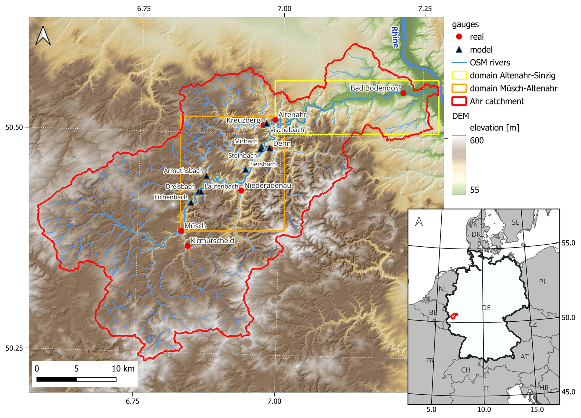
Figure 1 Ahr catchment, with major river network from OpenStreetMap (OSM), digital elevation model (DEM5), and locations of the real and virtual (model) gauges. Virtual gauges represent the locations where inflow boundary conditions from mHM to RIM2D are specified. RIM2D modelling domains Müsch-Altenahr and Altenahr-Sinzig are shown in orange and yellow boxes, respectively. Geodata: © GeoBasis-DE/BKG. © OpenStreetMap contributors 2024. Distributed under the Open Data Commons Open Database License (ODbL) v1.0.

3 Data and methods

3.1 Counterfactual precipitation fields

For the development of spatial counterfactuals, we use the E-OBS dataset v.25e of daily precipitation sums at a resolution of 0.11°×0.11° (Cornes et al., 2018), which extends until 31 December 2021 and includes the 2021 flood. For the purpose of hydrological modelling, the precipitation fields are regridded to the 0.0625°×0.0625° grid using bilinear interpolation. Since we focus on relative changes in flood characteristics between spatial counterfactuals, we expect the choice of this simple interpolation method not to notably affect the final results and conclusions. Furthermore, daily precipitation sums are disaggregated to hourly values using the method of fragments (Guan et al., 2023). A vector of hourly fragments, representing the relative distribution of hourly precipitation to the daily sum, is obtained from RADOLAN hourly observations. The RADOLAN dataset (Weigl and Winterrath, 2009; Winterrath et al., 2018) provides historical, hourly, Germany-wide, gridded, highly resolved precipitation data from a combination of the hourly values measured at climate stations with the precipitation recordings of 17 weather radars. The RADOLAN data have a spatial resolution of 1 km and cover the period from 1 June 2005 to the present. We use the coarser E-OBS data instead of directly applying RADOLAN hourly fields for two reasons. First, E-OBS contains consistent precipitation and temperature data needed for hydrological modelling. Second, the hydrological model used in this study is calibrated with the E-OBS data as part of the setup covering German catchments, including parts outside Germany, for which RADOLAN is not available.

The major trajectory of the atmospheric moisture transport into the affected region was from northeast to southwest on the northern flank of a low-pressure system (Mohr et al., 2023). Hourly precipitation footprints indicate that the Ahr catchment was only partly hit by the most extreme precipitation cells (Fig. 2). The 24 h precipitation totals inferred from the radar-based RADOLAN data product corroborate this observation (Mohr et al., 2023). The northwestern part of the catchment received the highest precipitation, but a large part of the extreme rainfall fell outside the catchment (Fig. 2). Comparison of the areas of the most intense precipitation (Fig. 2) with the orography (Fig. 1) reveals that these areas are not necessarily associated with high elevations in the Eifel mountains, but they are rather aligned with the major trajectory of the moisture transport. This suggests that the position of the trough, which controls the moisture transport, strongly influences the location of the precipitation footprint.

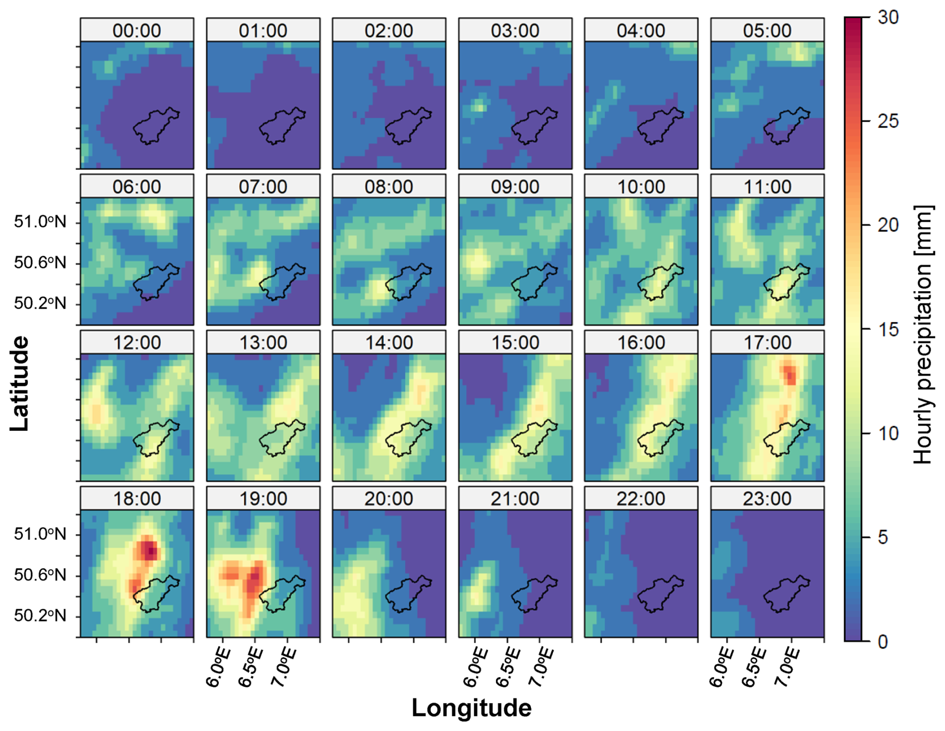
Figure 2 Hourly precipitation footprints from the disaggregated E-OBS dataset in the Eifel region around the Ahr catchment for 14 July 2021, between 00:00 and 23:00 UTC.

We develop spatial counterfactuals by shifting the entire precipitation field to the west and east, mimicking alternative positions of the low-pressure system. Additionally, we explore a few scenarios by shifting the precipitation footprint a few kilometres eastward and then southward (in a few steps). These counterfactuals mimic not only an alternative position of the trough, but also alternative scenarios of peak precipitation footprints along the major trajectory of moisture transport. We shift the precipitation field in steps of 0.0625°, corresponding to about 4.5 km at the latitude of the Ahr catchment (50° N). We explore precipitation shifts with 3 steps westward (W1, W2, W3) and 13 steps eastward (E1 to E13). Furthermore, after shifting the precipitation field five steps eastward, we investigate a range of steps along the north–south axis (E5N1–E5N4, E5S1–E5S5). The latter counterfactuals explore the effect of placing the most intensive precipitation between 18:00 and 20:00 UTC of 14 July 2021 centrally over the catchment (Fig. 2). In total, 25 scenarios are examined in addition to the reference scenario without shift (S0). The shifts are consistently applied to all hourly precipitation totals for the period of 5 d around the event date from 12 July 00:00 UTC to 18 July 2021 23:00 UTC.

3.2 Hydrological model

The hydrological response of the Ahr catchment to different spatial counterfactuals is investigated with the grid-based mesoscale Hydrologic Model (mHM) (Samaniego et al., 2010; Kumar et al., 2013; Samaniego et al., 2019), which is set up for the Ahr catchment with 3×3 km grid resolution and an hourly time step; mHM is driven by E-OBS precipitation fields disaggregated from daily to hourly values as described in Sect. 3.1. Hourly air temperature $T_j\left(j=\mathrm{1},\mathrm{2},\mathrm{\dots },\mathrm{24}\right)$ is disaggregated from E-OBS daily maximum (T_max) and minimum (T_min) air temperature using a cosine function (Förster et al., 2016):

$$\begin{array}{}\text{(1)}& T_j=T_{\min }+{\displaystyle \frac{T_{\max }-T_{\min }}{\mathrm{2}}}\left(\mathrm{1}+\cos {\displaystyle \frac{\mathit{\pi }\left(j+a\right)}{\mathrm{12}}}\right),\end{array}$$

where a controls the time of daily maximum temperature within a day. The value of a is calibrated based on observed hourly air temperature data and is set to 8 from January to April and 9 for other months for the study area.

The land surface characteristics required by mHM include a digital elevation model acquired from the Federal Agency for Cartography and Geodesy (BKG) and a digitized soil map from the Federal Institute for Geosciences and Natural Resources (BGR). Based on these maps, we extract information on soil texture properties, hydraulic conductivities, and topographic properties (such as slope, aspect, flow direction, and flow accumulation). Land cover information is derived from CORINE Land Cover scenes of the years 2000, 2006, 2012, and 2018 (European Environmental Agency, EEA), and mHM utilizes the multiscale parameter regionalization (MPR) (Samaniego et al., 2010) technique for consistent parameterization across space, resulting in a consistent parameter set for the entire model domain. The hydrological model is calibrated in a multi-site framework based on the dynamically dimensioned search (DDS) algorithm (Tolson and Shoemaker, 2007) using 6 years (2016–2021) of hourly discharge time series at gauges Müsch and Altenahr. Unfortunately, due to gauge failure, no instrumental records are available for the July 2021 event. We thus use the reconstructed flow hydrographs for model calibration considering high-water marks, inundation extents, and downstream gauge records as described by the Environment Agency of Rhineland-Palatinate (Berkler et al., 2022). We use the modified weighted Nash–Sutcliffe efficiency (wNSE) as the objective function, which puts a stronger weight on predicting high peak flows (Hundecha and Merz, 2012):

$$\begin{array}{}\text{(2)}& \mathrm{wNSE}=\mathrm{1}-{\displaystyle \frac{{\sum }_{i=\mathrm{1}}^N{Q}_{\mathrm{o}}\left(t_i\right){\left(Q_{\mathrm{s}}\left(t_i\right)-Q_{\mathrm{o}}\left(t_i\right)\right)}^{\mathrm{2}}}{{\sum }_{i=\mathrm{1}}^N{Q}_{\mathrm{o}}\left(t_i\right){\left(Q_{\mathrm{o}}\left(t_i\right)-\stackrel{\mathrm{‾}}{Q_{\mathrm{o}}}\right)}^{\mathrm{2}}}},\end{array}$$

where Q_o(t_i) and Q_s(t_i) are the observed and simulated discharges at time step t_i; $\stackrel{\mathrm{‾}}{Q_{\mathrm{o}}}$ is the mean observed discharge over the period of N time steps. Additionally, the Kling–Gupta efficiency (KGE), the Nash–Sutcliffe efficiency (NSE), and the percentage difference between the maximum simulated and reference discharge (i.e. observed or reconstructed) are used to characterize the model performance. Calibration and validation of hydrological models are typically performed using a split-sample approach (Klemeš, 1986). Since the July 2021 flood was an exceptional event, it should be included in both the calibration and validation. Given the presence of exceptional runoff conditions with widespread overland flow and very high runoff coefficients, it would be naïve to expect the model to capture such an event with parameters calibrated without this event. Finally, the validation should also include the 2021 flood, since this is the target event for the developed model. Hence, we need to adopt a different calibration and validation approach than a split-sample test. Here we use a spatial validation approach; we calibrate the model at gauges Müsch and Altenahr and validate the model at five gauges (Kreuzberg, Denn, Kirmutscheid, Niederadenau, and Bad Bodendorf; see Fig. 1) that are not used for calibration.

For the analysis of spatial counterfactuals, mHM is driven by different precipitation scenarios, whereas the temperature field is kept constant in space. Each mHM run uses a warm-up period of 5 years (2016–2020) prior to the July 2021 flood. The shifted precipitation field for the period of 5 d is inserted into the time series. Hence, spatial counterfactuals are applied to the factual simulated antecedent catchment conditions. Nevertheless, small deviations from the real antecedent soil moisture state occurs during the 5 d, where shifting is applied. They can be considered relatively small since no strong rainfall events occurred in this period.

3.3 Hydrodynamic model

We use the raster-based two-dimensional hydrodynamic model RIM2D which solves a simplified shallow-water equation. This so-called local inertia approximation disregards the convective acceleration term of the momentum equation and can be solved efficiently in the explicit manner (Bates et al., 2010). The inertia formulation has been previously evaluated in a number of synthetic tests (Bates et al., 2010) and real-case applications (e.g. Neal et al., 2011). Numerical instability occurring at supercritical flows can be efficiently tackled by introducing numerical diffusion, as proposed by de Almeida et al. (2012). RIM2D is coded in CUDA Fortran and parallelized for NVIDIA graphical processor units (GPUs). This efficient parallelization enabled long-term continuous simulations for flood risk assessments (Falter et al., 2015; Sairam et al., 2021) and paved the way for operational flood inundation and impact forecasting (Apel et al., 2022). In the latter study, Apel et al. (2022) set up the RIM2D model in a hindcast mode for the downstream part of the Ahr Valley, from gauge Altenahr down to the confluence with the Rhine. This setup forms the basis for the analysis presented in this study and was further extended upstream for the Müsch-Altenahr domain (Fig. 1).

RIM2D runs at a spatial resolution of 5×5 m. The topography is represented by the respective digital elevation model (DEM5), aggregated from the 1×1 m DEM of the federal state of Rhineland-Palatinate. The river channel bathymetry is poorly represented in DEM5; i.e. the bankfull depth is underestimated. The mean long-term water depth along the Ahr river is between 0.4 m at gauge Müsch and 0.85 m at gauge Bad Bodendorf. With water depths of up to 10 m during the July 2021 flood, Apel et al. (2022) showed that even the 10 m resolution is acceptable for simulating the inundation of this event. For the Altenahr-Sinzig reach, RIM2D exhibited a very high critical success index (CSI; Aronica et al., 2002) of 0.845 when run for event reanalysis driven by the reconstructed water depth hydrograph (Apel et al., 2022). The comparison of simulated and reported water depths also showed very good agreement: based on 75 high-water marks recorded at buildings in the inundated areas in the aftermath of the flood, the bias between reported and simulated water depth was −0.39 m, and the root mean squared error (RMSE) was 0.66 m.

The model domain used in Apel et al. (2022) is extended here to gauge Müsch, encompassing the entire Müsch-Sinzig reach (Fig. 1). The roughness parameterization of the RIM2D model is carried out based on the Mundialis (https://www.mundialis.de/en/germany-2020-land-cover-based-on-sentinel-2-data/, last access: 15 June 2025) land cover mapping for Germany, derived from Sentinel-2 data. The land use map is reclassified into seven classes; 12 different sets of Manning's values for these seven land use classes (Table S1 in the Supplement) are tested to find the best fit to the reconstructed flow hydrograph at gauge Altenahr.

Buildings are extracted from the OpenStreetMap (OSM) building layer, rasterized to the resolution of the DEM and overlaid with the topography. Hence, buildings are treated as impermeable obstacles in the hydrodynamic simulation; i.e. water flow is simulated around the buildings.

The upstream boundary condition for RIM2D is given by the hourly water depth hydrograph at gauge Müsch. The water depth is estimated from discharge time series simulated by mHM using the official gauge rating curve. The lateral inflow of the gauged tributaries Kirmutscheid, Niederadenau, Denn, and Kreuzberg is added by assigning the water depth hydrographs derived from the gauge rating curves from mHM discharges at the tributary mouths. For the nine ungauged tributaries (Fig. 1), synthetic rating curves are derived to convert mHM discharge to water levels using Manning's equation. The wetted perimeter, slope, and gauge datum (bed elevation) are derived from DEM5, and a roughness value of n=0.03 s m${}^{-\mathrm{1}/\mathrm{3}}$ is assumed. The resulting water level hydrographs are provided as lateral boundaries to RIM2D. At the downstream boundary, the normal depth condition is assumed; i.e. the water level gradient is the same across the domain boundary as for the previous two cells at the boundary. The two RIM2D simulation domains are initialized with steady-state conditions corresponding to the discharge just before the flood wave. For gauge Müsch, this was Q=9 m³ s⁻¹ (0.8 m water depth), which corresponds to the discharge recorded on 14 July 10:00 UTC. For gauge Altenahr, the discharge from the initial phase of the rising limb of the flood event with Q=130 m³ s⁻¹ (2.68 m water depth) at 14 July 17:00 UTC is used. The simulations are continued until a steady state is established and until the river channel represented by the DEM is filled.

3.4 Simulation experiments and evaluation procedure

All 25 spatial counterfactuals are simulated with mHM and RIM2D in addition to the reference scenario (S0). The mHM results in terms of peak flow and event volume are compared for all seven gauges in the Ahr catchment. From all simulations with RIM2D, we select two counterfactuals with the highest and lowest water levels at gauge Altenahr and compare them to the reference scenario. To evaluate the changes in the resulting inundation areas and maximum and mean water depths, we select 11 focus areas (Fig. 3) and compute the respective changes.

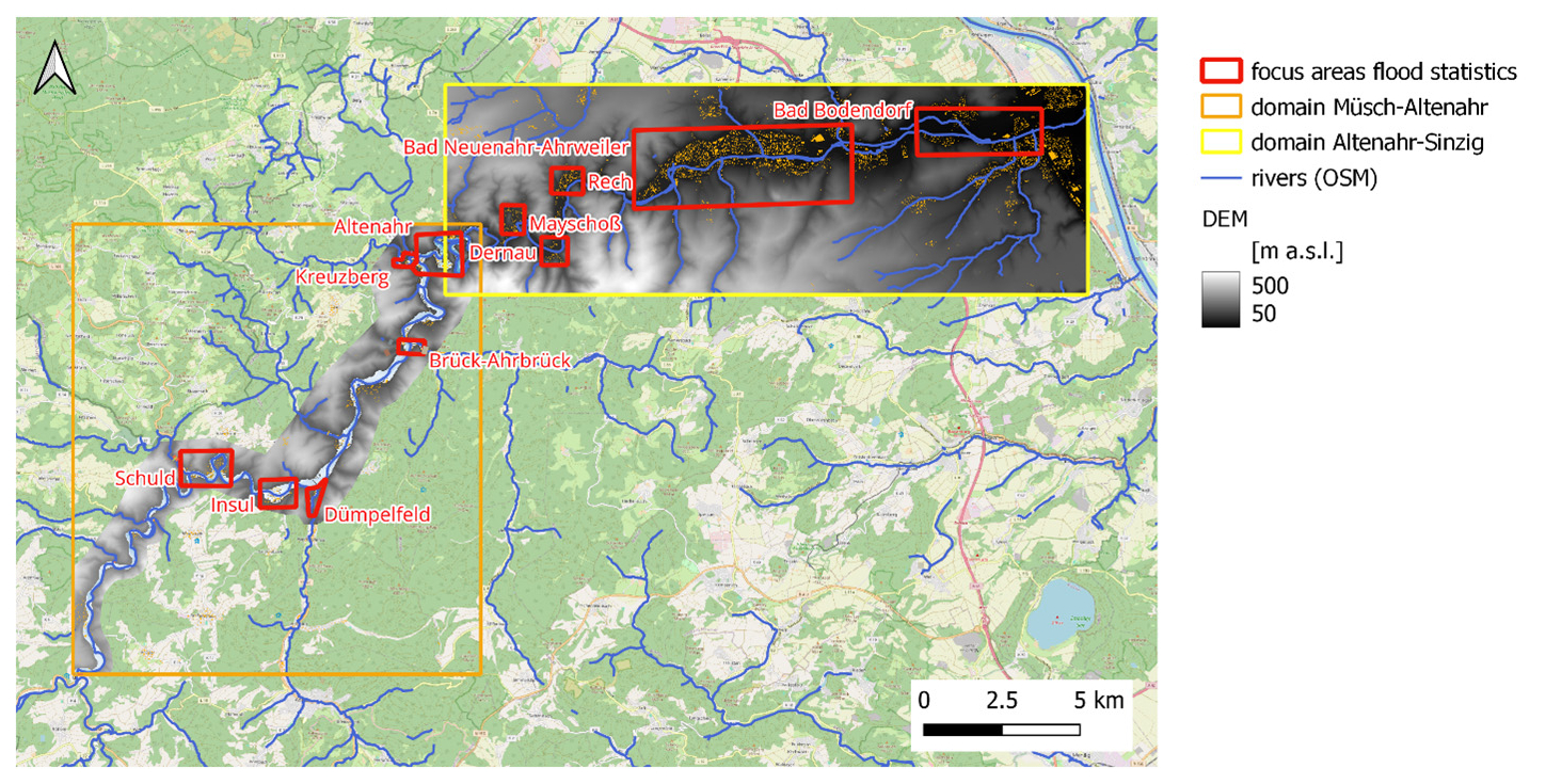
Figure 3 Overview of 11 focus areas used for evaluation of spatial counterfactuals with regards to inundation impact. These areas were particularly hit by the July 2021 flood. Geodata: © GeoBasis-DE/BKG. © OpenStreetMap contributors 2024. Distributed under the Open Data Commons Open Database License (ODbL) v1.0.

Table 1 Total maximum areal precipitation for 1, 3, 12, and 24 h durations and antecedent 2 d precipitation prior to 14 July 2021 0:00 UTC for all spatial counterfactuals and the reference scenario for the Altenahr catchment. Maximum values are in bold.

4 Results

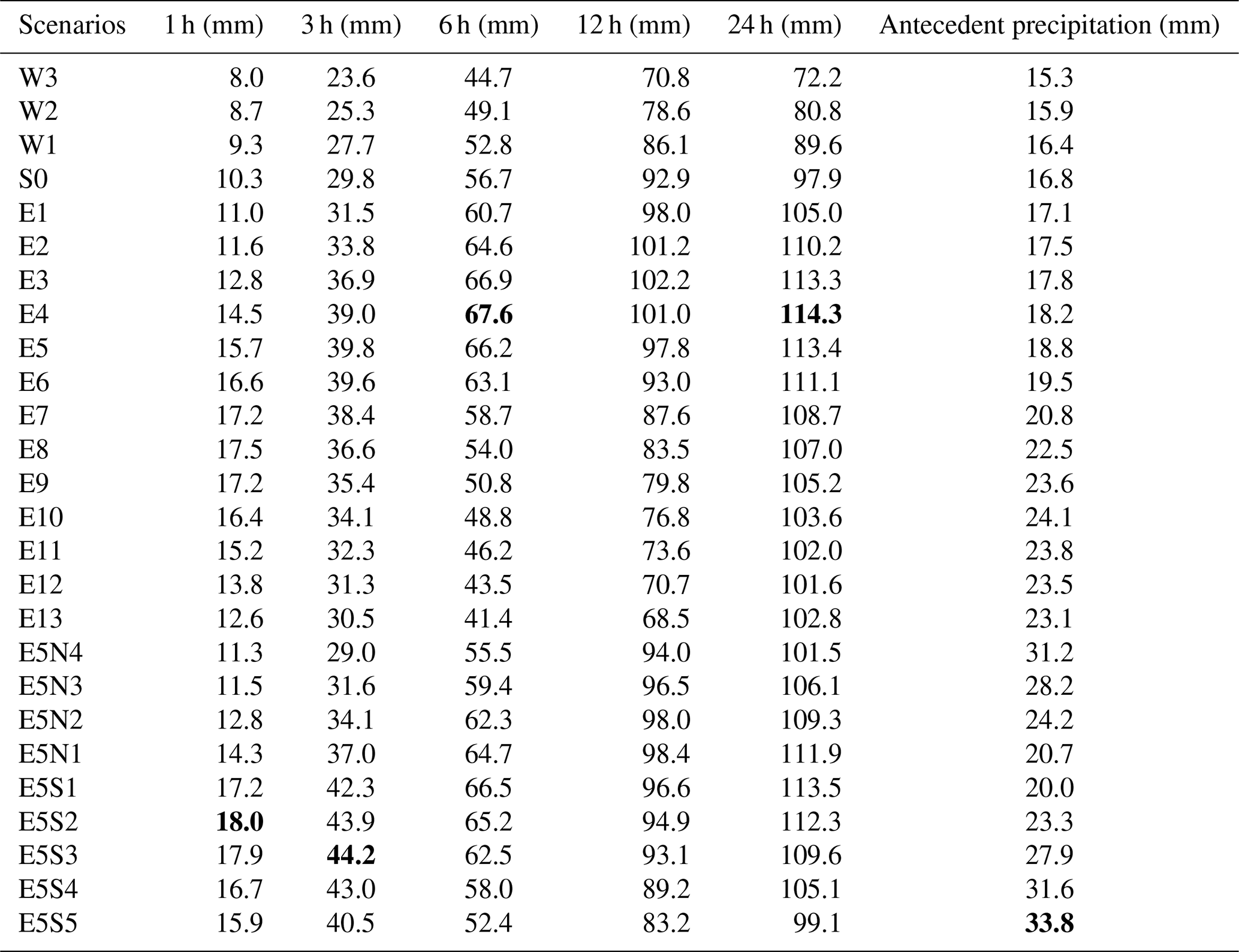
4.1 Antecedent and event precipitation in the counterfactual scenarios

For all scenarios, we compute the mean areal precipitation of the catchment gauged at Altenahr. We aggregate the event precipitation into 1, 3, 6, 12, and 24 h totals and find the maximum totals during the event (Table 1). Additionally, we aggregate the 2 d precipitation prior to 14 July 2021 to determine antecedent precipitation. For all counterfactuals with eastward shifting, we detect higher antecedent and event precipitation for all aggregation time windows compared to the S0 scenario. The westward shifts result in a gradual decrease in all precipitation indicators (Table 1). The scenarios E3 and E4 stand out as they exhibit the highest precipitation values at 6, 12, and 24 h aggregation steps.

4.2 Calibration and validation of the hydrological model

The calibration results for gauges Altenahr and Müsch over the period from 2016 to 2021 deliver wNSE values of 0.98 and 0.97, respectively. The validation performance at the other five gauges ranges with wNSE values between 0.35 at gauge Kreuzberg and 0.94 at gauge Bad Bodendorf. Figure 4 illustrates the model performance at the Altenahr gauge, including the hydrographs of the two largest floods within 2016–2021. The simulated streamflow shows a good agreement with the observations, especially for the high values including the 2021 flood event. The peak difference with the reconstructed data is only 7.8 %. Compared to the high wNSE value of 0.82 across all gauges, the average KGE and NSE values are relatively low at 0.59 and 0.57, respectively. This poorer performance mainly results from the overestimation of the low flow by the model.

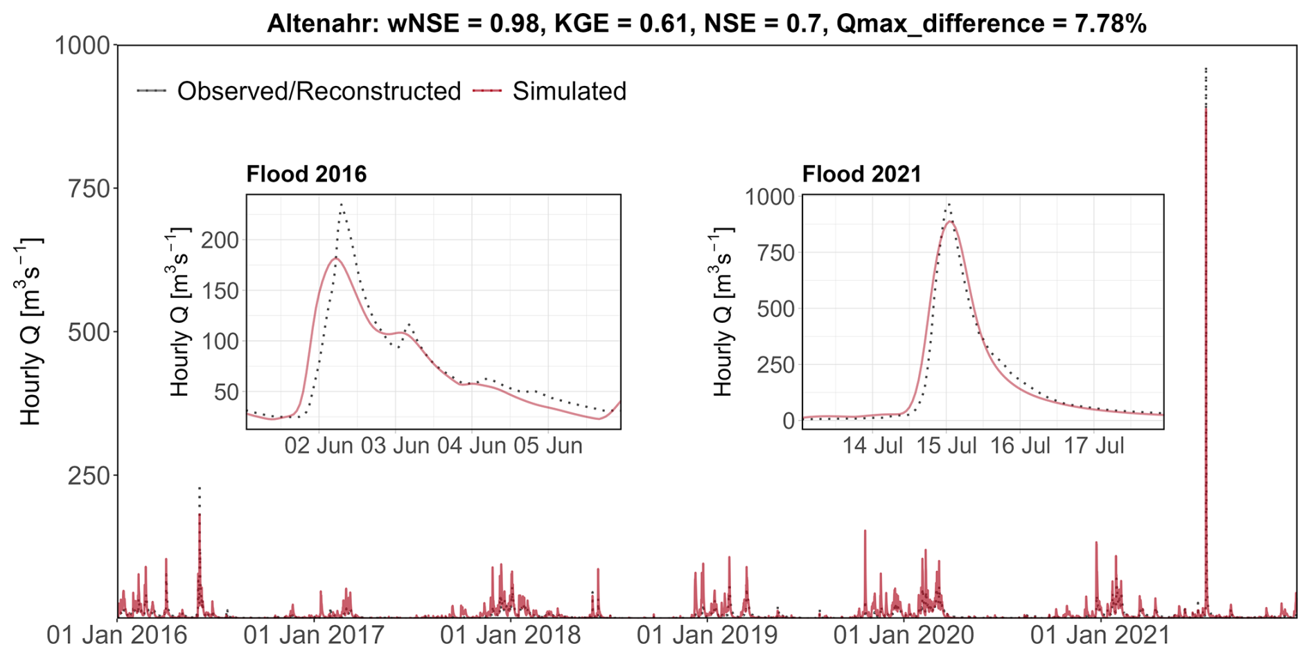
Figure 4 Simulated and observed/reconstructed discharge (Q) time series for gauge Altenahr during 2016–2021. Two insets display the hydrographs for the two largest recorded flood events in June 2016 and July 2021.

4.3 Discharge in the counterfactual scenarios

All spatial counterfactuals are evaluated in terms of changes in flood peak and flood event volume with respect to the reference scenario (S0) at the seven gauges (Fig. 5). The flood volume is computed for the event duration from 13 July 00:00 UTC to 18 July 23:00 UTC. For comparison, the reconstructed event is also plotted in the volume/peak change diagrams. For every sub-catchment, we find scenarios that result in both a larger peak flow and a larger event volume compared to the reference scenario (S0). The maximum changes are simulated at gauge Denn, reaching nearly 160 % increase in peak flow and around 90 % increase in event volume for the E7/E8 counterfactuals. Besides Denn, other sub-catchments located in the southeastern part of the Ahr catchment, including Kirmutscheid and Niederadenau, exhibit a strong reaction with more than 75 % and 100 % change in peak flow, respectively. In these two tributaries, the counterfactuals with eastward and southward shifts caused the highest peaks (E5S2/E5S3). The least sensitive sub-catchment is Müsch, with maximum peak and volume increases of about 20 %. With a westward precipitation shift, the peak flow decreases up to 30 % (W3). The precipitation footprint in the reference scenario (S0) shows already intensive rainfall in the northwestern part of the Ahr catchment (Fig. 2) and represents one of the worst scenarios for the Müsch sub-catchment when compared to the shifted patterns. The westward shifts (W1–W3) result in gradual and nearly proportional reduction of peak and volume in all sub-catchments. Gauge Denn shows here the most sensitive response, with a reduction of up to 60 % (Fig. 5).

In several small sub-catchments, i.e. Denn, Niederadenau, Kirmutscheid, and Kreuzberg, the counterfactuals are strongly aligned along a bisecting line. The larger sub-catchments Müsch, Altenahr, and Bad Bodendorf are less sensitive and show a more mixed response; i.e. the points form clouds rather than a line (Fig. 5). The linear response is observed in the tributaries, while the mixed response is simulated for gauges at the main stream. In small catchments, the stronger the overlap between the precipitation footprint and the catchment area, the stronger the response. In larger catchments, the inflow from different tributaries is mixed, and the entire reaction is dampened.

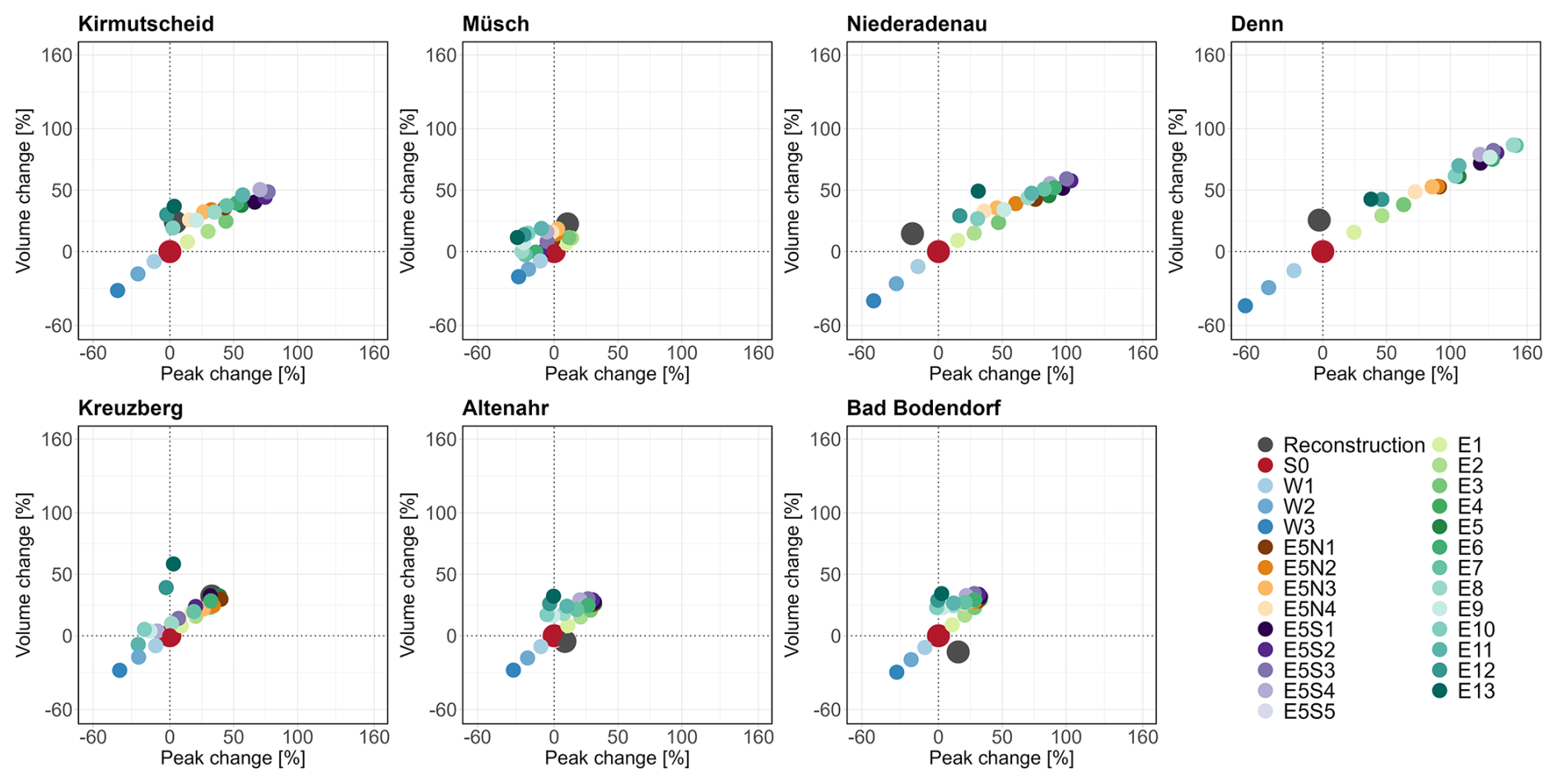
Figure 5 Simulated changes in the flood peak and volume in the counterfactual scenarios as compared to the reference scenario (S0) at seven gauge locations in the Ahr catchment.

The worst counterfactuals in terms of maximum peak or volume changes are different for different sub-catchments. There is no single worst-case scenario for all tributaries that causes the worst case in the main channel. Further, there is no single clear sequence of counterfactuals with increasing order of response (increasing peak and volume) valid for all tributaries that would translate into a similar sequence of counterfactuals for gauge Altenahr. However, in general, eastward shifts of the precipitation by about 13.5 to 22.5 km (E3–E5) with some additional southward shifts (E5S1–E5S5) result in the highest peaks in almost all tributaries.

Figure 6 looks closer at gauge Altenahr upstream of the major town Bad Neuenahr-Ahrweiler, where widespread inundation and impacts occurred in July 2021. The worst counterfactual in terms of flood peak change is E5 (eastward shift of about 22.5 km), which results in an increase of 32 % and a corresponding flood volume change of 26 %. Several other counterfactuals result in peak flow changes that are only a few percentage points lower (E3 (28.5 %), E5S1 (31.5 %), E5S2 (30 %)). These scenarios exhibit the highest areal precipitation in the Altenahr sub-catchment at various timescales (Table 1). Particularly, the E3 scenario has the highest 6 and 12 h precipitation values. Many counterfactuals with eastward shifts of only a few kilometres result in peak and volume increases of more than 10 %. The strongest volume increase of 32 % (E13) is not much larger than in the highest-peak counterfactual (E5, 28 %) (Fig. 6). The E13 scenario, however, delivers a small reduction of peak flow by 0.5 %.

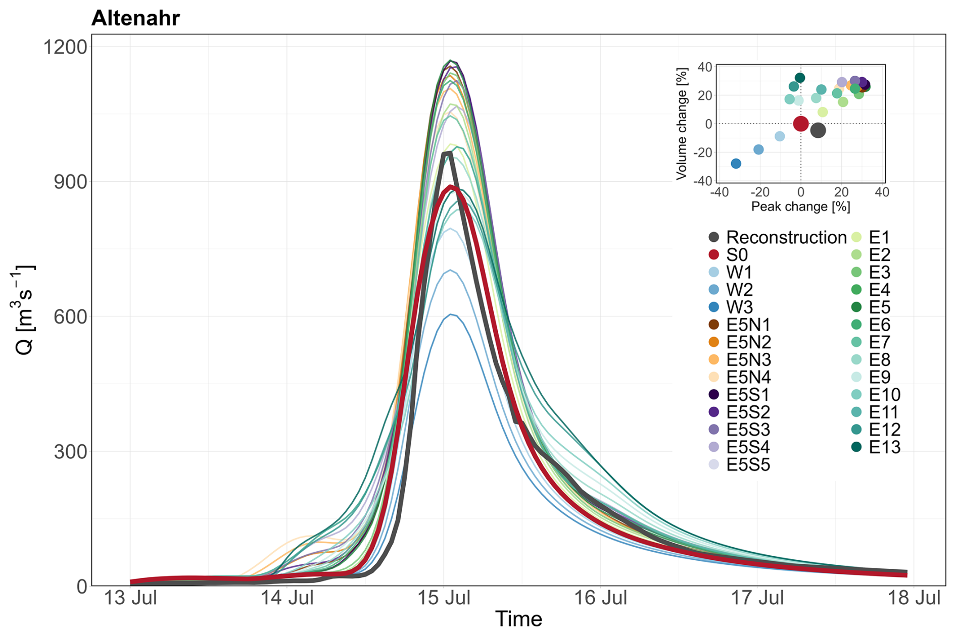
Figure 6 Flood hydrographs for the simulated reference scenario (S0) and spatial counterfactuals, as well as the reconstructed flood hydrograph of the July 2021 flood at gauge Altenahr. The inset displays the peak/volume change diagram for various scenarios.

4.4 Calibration and validation of the hydrodynamic model

The RIM2D model is manually calibrated by testing 12 different parameter sets and comparing the resulting water level hydrographs to the hydrograph reconstructed at gauge Altenahr (Fig. 7). RIM2D is driven by the water level hydrograph at gauge Müsch as an upstream boundary condition. This hydrograph is derived from the calibrated mHM flow simulations that are converted to water levels using the rating curve at gauge Müsch. Lateral inflows from the tributaries are considered, as described in Sect. 3.3.

We select the calib4 parameter set (Table S1) as it provides the best match between the simulated and reconstructed water level hydrograph at gauge Altenahr when using mHM output as boundary conditions for the RIM2D model of the Müsch-Altenahr reach (Fig. 7). This parameter set is further used to simulate spatial counterfactual inundations. The calibrated RIM2D simulation shows higher initial water levels because of the assumed higher initial water depths and overestimates the water depths by 0.13 m, with an earlier rise of the flood limb compared to the reconstruction. On the contrary, the mHM hydrograph shows a stronger attenuation and lower peak of 0.55 m. This can in part be explained by the simple kinematic wave routing used in mHM and by uncertainty introduced by applying an extrapolated rating curve at gauge Altenahr to convert the mHM-simulated flows into water levels.

For the lower reach of Altenahr-Sinzig, a dedicated roughness calibration was performed by applying a Monte Carlo sensitivity analysis (Khosh Bin Ghomash et al., 2025). From this study, the best-performing roughness dataset for simulating inundation extent, water level in the river, and water depth in the floodplain was selected to simulate the counterfactual inundation in this reach.

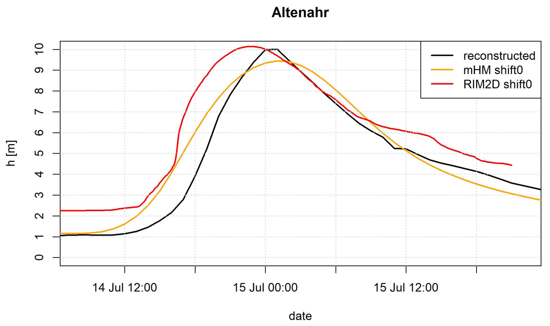
Figure 7 Water depth (h) hydrographs: reconstructed gauge record, simulated by RIM2D using the best roughness parameter set (calib4), mHM S0 discharge simulation at the gauges in the Müsch-Altenahr reach, and the simulated discharge at Altenahr by mHM converted to the water depth hydrograph using the extrapolated rating curve at gauge Altenahr.

4.5 Inundation in the counterfactual scenarios

We simulate inundation dynamics for all 25 spatial counterfactuals as well as for the reference scenario S0. Different counterfactuals result in different maximum water levels and inundation areas at different locations along the Ahr river. At gauge Altenahr, for example, the maximum water level between the counterfactual scenarios simulated by RIM2D ranges between 169.20 and 172.70 m a.s.l., which is around 169.19 m a.s.l. corresponding to scenario S0 (Fig. 8). The span between the maximum water levels of the counterfactuals is 3.5 m, indicating how much less or more severe the flood could have been with shifting rainfall fields. In the RIM2D simulations, the highest water level is reached in scenario E3 and the lowest one in W3. These counterfactuals are selected for further detailed analysis of changes in inundation. The range of maximum water levels converted from the mHM discharge simulations is 4.32 m, which is somewhat larger compared to RIM2D (Fig. 8). In the mHM ensemble of counterfactuals, the largest peak at gauge Altenahr is obtained in E5 and the lowest in W3. As explained earlier, the different routing schemes, underlying data, and conversion of discharge to water levels for mHM influence the ordering of the counterfactual scenarios, although the differences are small, e.g. the difference between the E3 scenario run with RIM2D routing and the E5 scenario run with mHM and converted to water level amounts to 0.52 m (Fig. 8). Since we analyse relative changes between counterfactuals, this difference is not expected to notably affect the final results and conclusions.

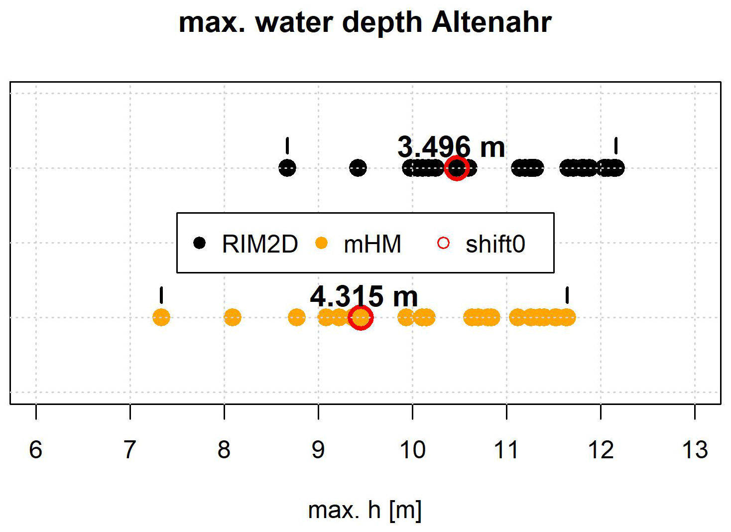
Figure 8 Comparison of maximum water depths (h) at gauge Altenahr simulated with RIM2D and mHM discharge concerted by the gauge rating curve. “shift0” indicates the actual flood event with no shift of the rainfall field.

The strong discrepancy in lower water levels between RIM2D and the reconstructed scenario can be explained by assumed initial water depths in the RIM2D model, which are higher than the water levels in the Ahr before the rise of the flood hydrograph. This initial water depths were set that high to ensure a continuous flow in the river channel, where bed elevation is not properly represented in the unmodified 5m DEM. Nevertheless, the peak water levels are comparable, as the effect of the high initial water depth fades out with increasing water depths. In the previous study by Apel et al. (2022), the maximum water depths in the inundated floodplains between Altenahr and the Ahr outlet were also shown to match well with field records. The higher water depths at the onset of the flood event may contribute to higher celerity in the RIM2D simulations, resulting in an earlier flood peak compared to the reconstructed one.

In the following step, we analyse the resulting differences in mean and maximum water depths as well as the difference in flooded area between the reference scenario (S0) and the two counterfactuals W3 and E3 (Table 2, Figs. 9–11, A1–A4). The fact that both W3 and E3 counterfactuals correspond to the same shift of the precipitation footprint by about 13.5 km, but in opposite directions, allows us to investigate the sensitivity of inundation characteristics to these shifts.

Table 2 Differences in mean and maximum simulated water depth (h) and flooded area between the reference scenario and the spatial counterfactuals resulting in the highest (E3) and lowest (W3) maximum water depth at gauge Altenahr.

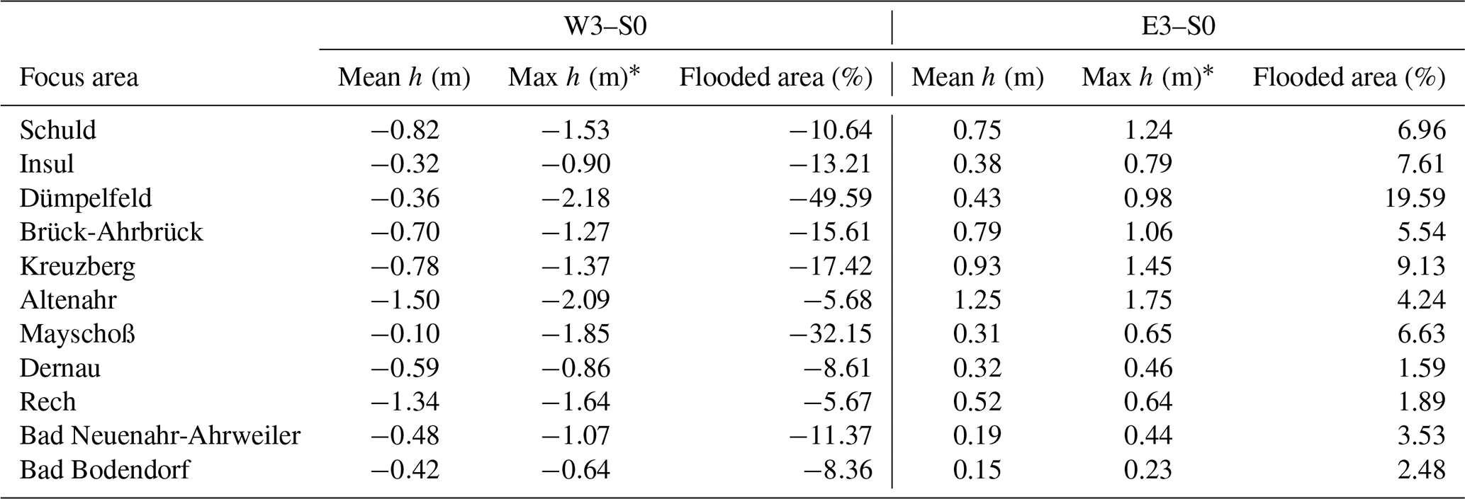
^* Max h gives the 99.99 percentile of water depths to avoid potential biases by spurious maximum water depths caused by numerical instabilities and/or DEM errors.

The results are presented for 11 selected focus areas. For all areas, E3 leads to a consistent increase in all three inundation characteristics, whereas W3 results in a consistent decrease. In the E3 scenario, the mean and maximum water depths are 1.25 and 1.75 m higher, respectively, than in S0 in the area of Altenahr. In the adjacent area at Kreuzberg, these numbers reach 0.93 and 1.45 m. In these topographically constricted areas, changes in inundated areas are relatively small around 4 % and 9 % (Table 2, Fig. 9).

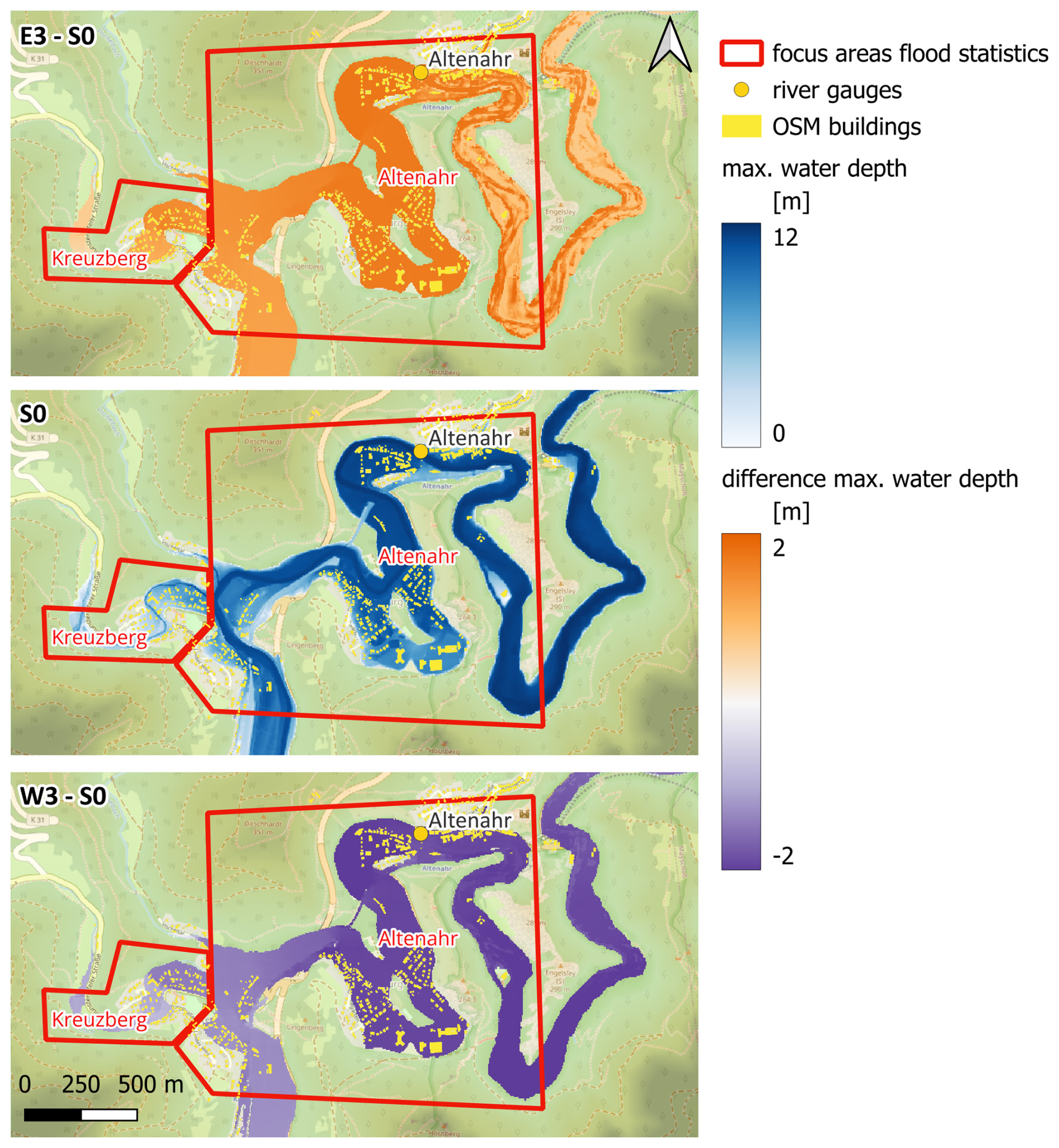
Figure 9 Inundated area and maximum water depths in the focus areas of Altenahr and Kreuzberg for the reference scenario S0 as well as differences between E3 and S0 (E3–S0) and between W3 and S0 (W3–S0) scenarios. © OpenStreetMap contributors 2024. Distributed under the Open Data Commons Open Database License (ODbL) v1.0.

The largest increase in the flooded area of nearly 20 % in E3 is detected in the village of Dümpelfeld at the mouth of the Adenauer Bach tributary (Fig. A1). Here, also the maximum water depth is higher by nearly 1 m compared to S0. This focus area also shows the largest inundation area decrease of nearly 50 % in the W3 scenario. The Adenauer Bach catchment has a distinct north–south orientation (Fig. 3). Hence, it becomes highly sensitive to the shifts in the precipitation footprint along the east–west axis. Three focus areas that were severely hit by the flood and experienced large damages – Schuld, Insul, and Brück-Ahrbrück – also show a relatively high sensitivity of the inundation indicators to the east–west shifting (Figs. A1 and A2). Particularly at Schuld, with a narrow, deeply incised valley, the mean and maximum water depths show strong variations between E3, S0, and W3 (Table 2).

In Mayschoß, the eastward shift results in a comparatively modest increase in inundation area of about 7 % and an increase in mean and maximum water depths of 0.31 and 0.65 m, respectively, compared to S0 (Table 2). However, W3 results in a dramatic relief for this focus area: the inundation extent is reduced by 32 %, since the settlement area in the southern part of the village is entirely spared from flooding (Fig. 10). The sensitivity of the inundation indicators reduces substantially downstream of Altenahr and Mayschoß in the areas of Dernau, Bad Neuenahr-Ahrweiler, and Bad Bodendorf with the exception of Rech (Table 2, Figs. 10–11, A3–A4).

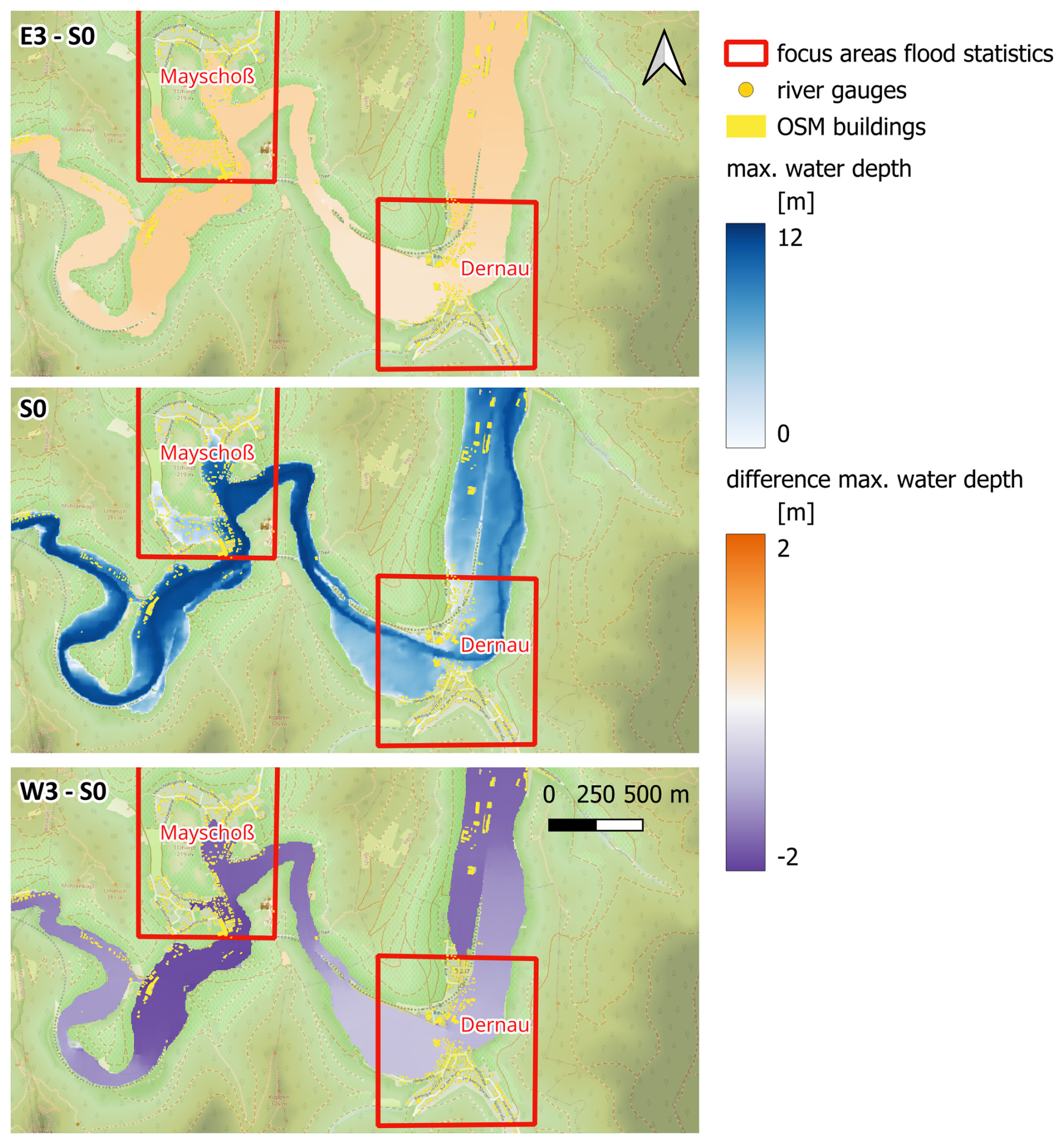
Figure 10 Inundated area and maximum water depths in the focus areas of Mayschoß and Dernau for the reference scenario S0 as well as differences between E3 and S0 (E3–S0) and between W3 and S0 (W3–S0) scenarios. © OpenStreetMap contributors 2024. Distributed under the Open Data Commons Open Database License (ODbL) v1.0.

In the downstream areas with wider floodplains at Bad Neuenahr-Ahrweiler and Bad Bodendorf, the simulated changes in inundated areas and water depths are comparatively small between the analysed counterfactuals. Mean water depth differences vary between −0.48 m and 0.19 at Bad Neuenahr-Ahrweiler and between −0.42 and 0.15 m at Bad Bodendorf. These two focus areas experienced the highest number of flood victims in the Ahr catchment. Although the increases in inundation areas and flood depths are not dramatic for E3, the relief for the comparable westward shift is stronger but still smaller compared to other focus areas (Table 2, Figs. 11,  A4). Here, most of the settlement areas remain exposed to floodwaters. The lower sensitivity of the downstream areas can be expected, as they integrate the discharge from different tributaries and parts of the catchment. So, lesser precipitation input and less severe flooding in some sub-catchments is compensated by more severe flooding of the others.

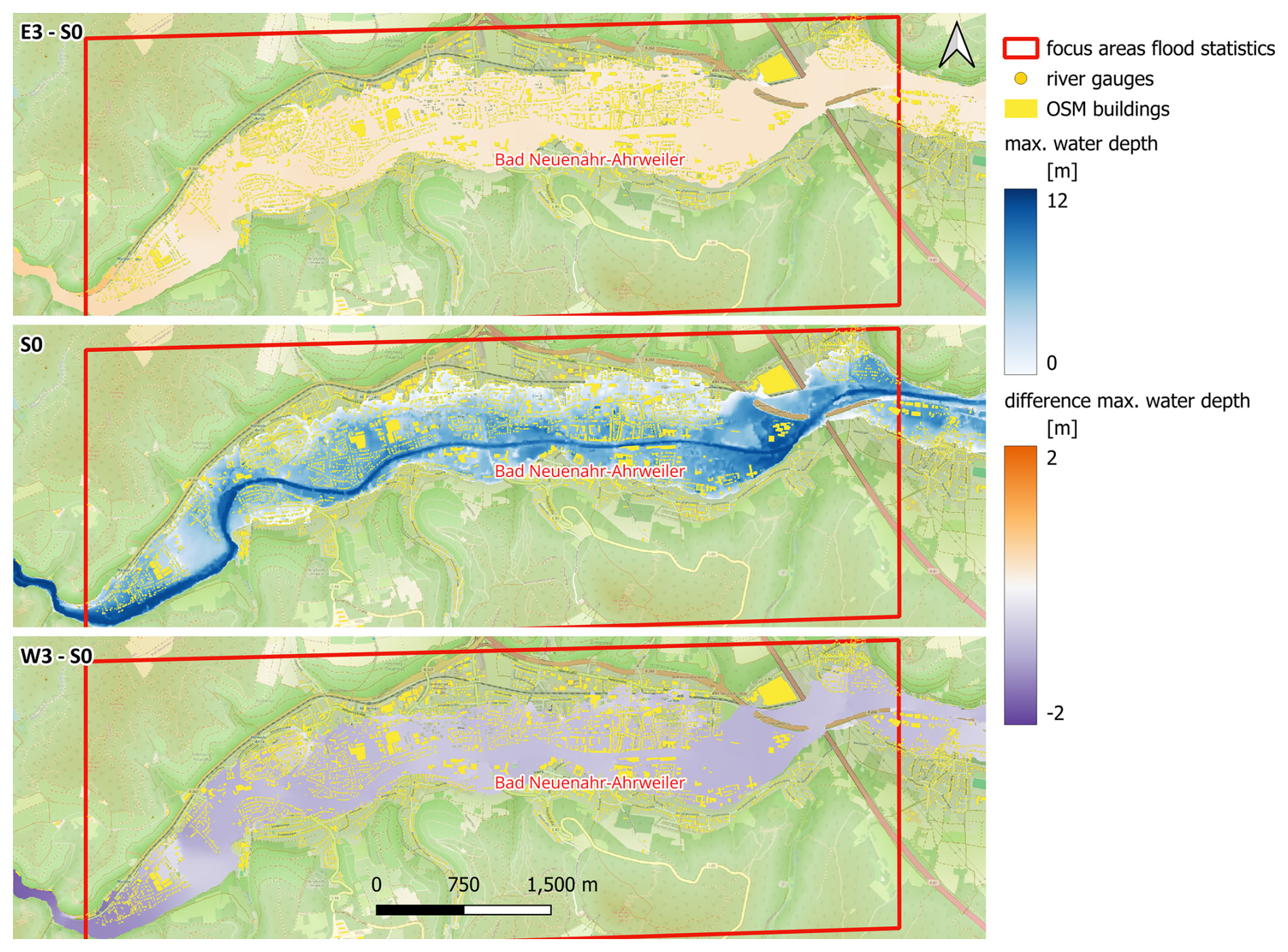
Figure 11 Inundated area and maximum water depths in the focus area of Bad Neuenahr-Ahrweiler for the reference scenario S0 as well as differences between E3 and S0 (E3–S0) and between W3 and S0 (W3–S0) scenarios. © OpenStreetMap contributors 2024. Distributed under the Open Data Commons Open Database License (ODbL) v1.0.

4.6 Impact in counterfactual scenarios

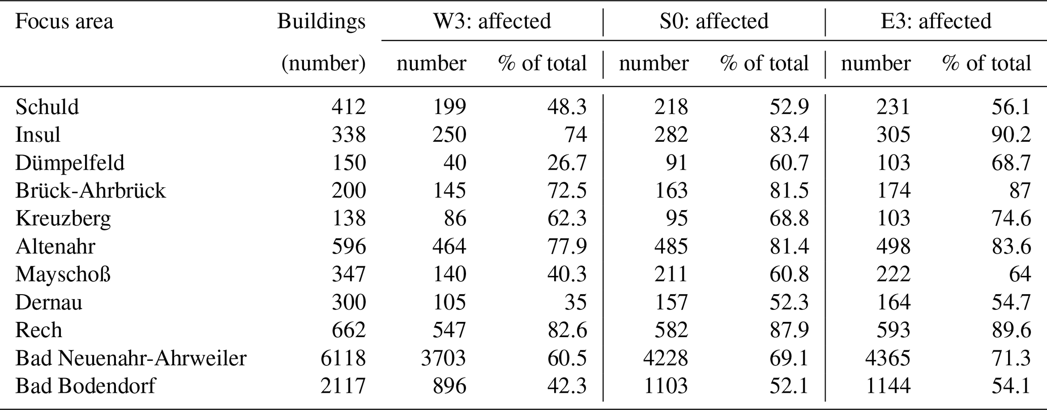
Table 3 shows the affected buildings in the focus areas for the W3, S0, and E3 scenarios. Affected buildings are determined by buildings whose footprint plus a buffer of 2 m around the footprint have a mean inundation depth above 0.0 m. The buffer was used because the footprints are rasterized to 5 m resolution, thus losing some detail, and because the footprints are excluded from the hydraulic simulations, thus always showing inundation depths of 0.0 m in the rasterized representation. The percentage of affected buildings in the focus areas ranges from 52.1 % at Bad Bodendorf up to 87.9 % at Rech (Table 3). These numbers increase from 54.1 % at Bad Bodendorf to 90.2 % at Insul in the E3 scenario. The range of the affected buildings between the scenarios depends not only on the topography of the individual focus areas, but also on the different tributary discharge and consequent inundation. In the case of Dümpelfeld, the large difference in inundation is caused by the much higher discharge of the tributary brook Adenauer Bach in E3. In this case, the fire station is also affected, which was not the case during the actual event (Fig. 12). The inundation depth is moderate (around 0.2 m), but this could have impaired the responsiveness of this fire station.

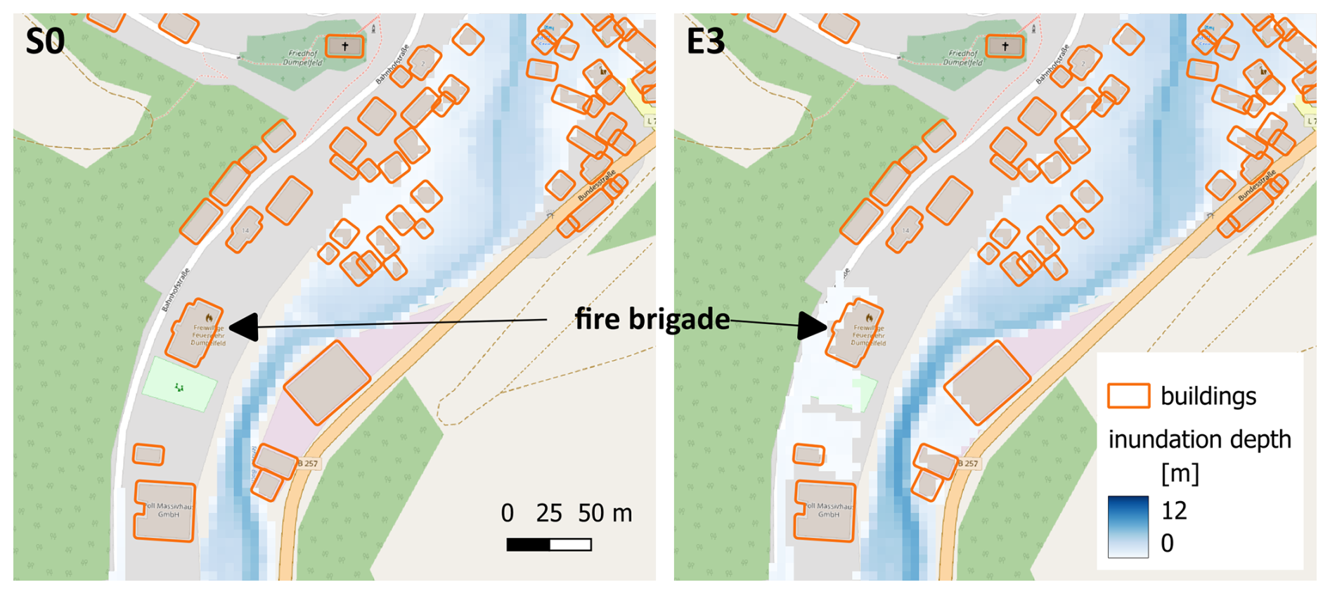
Figure 12 Maximum inundation depths in scenarios S0 (left) and E3 (right). Inundation around the fire station in Dümpelfeld is about 0.2 m in the E3 scenario. Building footprints shown are OSM footprints buffered with 2 m. © OpenStreetMap contributors 2024. Distributed under the Open Data Commons Open Database License (ODbL) v1.0.

Table 3 Number and percentage of affected buildings in the focus areas for the least (W3), reference (S0), and most severe (E3) counterfactual scenarios.

5 Discussion

The present analysis suggests that the Ahr flood catastrophe could have easily turned out much worse if the trajectory of atmospheric moisture flow and the precipitation footprint were shifted just 10–20 km eastward. This trajectory was primarily controlled by the atmospheric circulation and the position of the low-pressure system. We could not observe a notable effect of orography on the emergence of areas of particularly heavy precipitation in the Ahr catchment. Hence, the explored shift seems to be realistic and may occur in the future. The overall low probability of such an extreme event still has to be kept in mind (Kreienkamp et al., 2021; Vorogushyn et al., 2022).

The hydrologic response of the sub-catchments to the imposed spatial counterfactuals is strikingly different. In small sub-catchments, we simulate much higher peak flows of up to 160 % at gauge Denn compared to the reference scenario S0. In larger sub-catchments, the response is weaker but still notable. For example, at gauge Altenahr, we simulate about 32 % higher peak discharge for an eastward shift of about 20 km. The same event generates a more than 20 % higher flood event volume (Fig. 6). A similar maximum increase in peak flow at gauge Altenahr by about 30 % was found by Voit and Heistermann (2024a), who applied a much broader range of spatial counterfactuals. Thus, this value seems to be the maximum peak flow enhancement that can be achieved by shifting such an event in space. Other modifications of the observed precipitation event are possible, such as a rotation of the precipitation footprint or changes in the overall intensity or the spatio-temporal structure. Voit and Heistermann (2022) noted that precipitation intensities can cause floods at different spatial and temporal scales. Hence, by modifying the overall spatio-temporal structure of the precipitation, an even stronger response cannot be ruled out. In addition, higher precipitation intensities are likely to occur in a warmer climate (Kreienkamp et al., 2021; Tradowsky et al., 2023; Ludwig et al., 2023). Such changes in precipitation may be amplified by a non-linear runoff generation response, e.g. when the prevailing flood generation process changes to faster overland and subsurface flow with increasing rainfall intensities (Rogger et al., 2012; Macdonald et al., 2024). Hence, the non-linear exacerbation of peak runoff, e.g. as projected by Ludwig et al. (2023) of up to 39 % at gauge Altenahr for a +2 °C warmer climate, can be even further aggravated by an unfavourable spatial counterfactual.

The hydrodynamic response to the spatial counterfactuals varies between the locations along the river. We observe different sensitivities of water depth and inundation extent at different locations to comparable shifts along the east–west axis. Small tributaries show a strong response in water depth and inundation extent at the confluence into the main channel. As can be expected from morphological characteristics, mean and maximum water depths exhibit a strong sensitivity in constricted incised valleys. In the wider floodplains of the downstream areas at Bad Neuenahr-Ahrweiler and Bad Bodendorf, the differences in water depths between the counterfactuals are comparatively small. The strongest response of mean and maximum water depths is simulated around Altenahr. Here, shifts of the precipitation footprint in east and west directions by about 10–15 km result in changes in mean and maximum water depths by about −1.5 to +1.25 and −2.1 to +1.75 m, respectively. In the area around Altenahr, the flow from all major tributaries is concentrated in a relatively narrow valley, before the flood wave propagates further downstream and attenuates on wider floodplains at Bad Neuenahr-Ahrweiler and Bad Bodendorf. The significant increase in maximum water depths in the worst counterfactual raises the number of affected buildings and can also potentially affect critical infrastructure such as fire station involved in catastrophe management. Hence, spatial counterfactuals are helpful for planning and securing the operation of critical services in advance of unprecedented floods.

The use of the hydrologic and hydrodynamic models for the analysis of spatial counterfactuals is associated with uncertainties in model structure as well as input data and parameterization. We, however, analyse relative differences in flood characteristics between various scenarios. Hence, the effect of uncertainty is expected to be fairly limited on the final results and conclusions, and we do not explicitly consider these uncertainties in the presented analysis. Interestingly, Voit and Heistermann (2024a) found a very similar maximum relative increase in flood peak for the Ahr flood using a different hydrological model and completely different approach to construction of counterfactuals. This confirms our expectation. In fact, we can view the analysis of spatial counterfactuals as an exploration of aleatory uncertainty (natural variability) in spatial precipitation footprints.

Here, we analyse only a limited number of spatial counterfactual scenarios, 25 in total. Precipitation fields are shifted in discrete steps of 0.0625° in fixed directions primarily along the west–east axis and at the fifth step eastward along the north–south axis. We selected these scenarios after visual analysis of precipitation fields, aiming at maximizing the total precipitation input over the Ahr catchment. There is no guarantee that some other scenarios exist that might cause even higher peak flows and stronger inundation at specific locations. The number of spatial counterfactuals is virtually infinite. Our aim, however, is not to identify the worst-case scenario but rather to explore a computationally feasible set of unprecedented events. In search of unprecedented events, Merz et al. (2024) also considered 24 spatial counterfactuals for each of the past 10 most damaging floods in Germany. They performed systematic shifts in eight azimuthal directions and with much larger radii (20, 50, and 100 km) compared to our approach. Voit and Heistermann (2024a) relaxed the spatial constraints even further by shifting the past 10 most severe precipitation events to match the centroids of more than 22 000 sub-catchments across Germany. Theoretically, even in these two cases the existence of an uncovered worst-case counterfactual cannot be ruled out.

Shifting past rainfall events to different areas raises concerns about the plausibility of the occurrence of such events. This depends on the type and strength of the precipitation events as well as the moisture transport patterns and their interactions with orography. Recently, Voit and Heistermann (2024b) compared global and local spatial counterfactuals for generating synthetic floods in small basins in Germany. Global counterfactuals were based on shifting high-precipitation events across the whole of Germany, whereas local counterfactuals were constructed by shifting the events within a 20 km buffer around a catchment of interest in Germany. As could be expected, global counterfactuals can produce more extreme floods than local counterfactuals, but credibility of such scenarios becomes questionable with increasing transposition distance. Although the question about the reasonable transposition distance remains open, Voit and Heistermann (2024b) demonstrated that already from high-precipitation events within a small radius of 20 km an alarming number of plausible flood events exceeding 50- and 200-year return periods can be generated for a catchment of interest. It is clear that the further away a precipitation event is shifted, especially into different topographic and climatic settings, the more questionable the plausibility of its occurrence becomes. This issue can be addressed, for example, by shifting the event the triggering circulation pattern in a climate model and letting the event develop under slightly different initial conditions but constrained by the actual orography. Perturbations to past events to construct future weather are typically applied to explore how the event would unfold under warmer conditions (e.g. Manola et al., 2018; Ludwig et al., 2023). Similar experiments can be conceived in a stationary climate but applying spatial counterfactuals to circulation dynamics. This approach introduces additional uncertainties through a climate model and requires additional computational effort. Also, the resulting events would not be strictly spatial transposition of the past precipitation footprints but would unfold their own spatio-temporal dynamics. Further relaxing meteorological constraints, stochastic generation of event sets by modifying specific characteristics of the past observed events (e.g. spatial extent, total rainfall volume, and peak intensity, considering their marginal statistics) can be considered, following the approach by Diederen and Liu (2020).

Our approach limits the number of spatial counterfactuals due to computational constraints and evaluation effort. We do not seek to find the worst possible spatial counterfactual, which may even be far from the probable maximum flood, i.e. the worst possible flood. We rather argue that even small changes in moisture flow and shifts of precipitation fields by a few kilometres may cause even more severe consequences than have been experienced. Our results should alert emergency and flood risk managers as well as the general public that the past catastrophe was not the worst possible flood but could have easily turned out worse and thus may occur as such in the future.

The approach of spatial counterfactuals is charming from the perspective of flood risk communication as it can be easily explained and demonstrated to flood risk professionals as well as the general public. The approach is based on perturbing an actual past precipitation or flood event which is familiar to most people in the affected communities. Hence, people can imagine more easily the possibility of even worse catastrophe dynamics and impacts. This will hopefully increase their willingness to undertake risk reduction measures for unprecedented events.

6 Conclusions

In the presented paper, we use the approach of spatial counterfactuals to explore unprecedented floods. By systematically shifting in space the footprint of the precipitation event, which caused the deadly July 2021 flood in the Ahr catchment in Germany, we simulate the resulting flood peaks, inundation areas, and maximum depths as well as exposed assets. Our findings suggest that the 2021 flood catastrophe could have been even worse if the atmospheric moisture trajectory hit the catchment only 15–25 km further east. In this case, we simulate peak flows at gauge Altenahr of about 32 % higher compared to the simulation of the actual flood. This increase in peak is associated with an increase in flood event volume of 26 %. In some small tributaries, an increase in peak flows of up to 160 % is simulated in these counterfactuals. The resulting differences in inundation extents and depths vary along the valley, depending on counterfactuals and topographic properties of specific areas. For example, in a focus area around Altenahr, the mean and maximum inundation depths increase by 1.25 and 1.75 m, respectively, in the worst simulated scenario. We demonstrate that considerably more assets could have been affected by a counterfactual flood, including some critical infrastructure such as a fire station. We encourage the use of spatial counterfactuals for informing flood risk professionals as well as the general public on potential unprecedented events, thus fostering better precaution and flood risk management in the years to come.

Appendix A

Table A1 Parameter sets of Manning's roughness coefficients for different land use classes used for calibration of the RIM2D model.

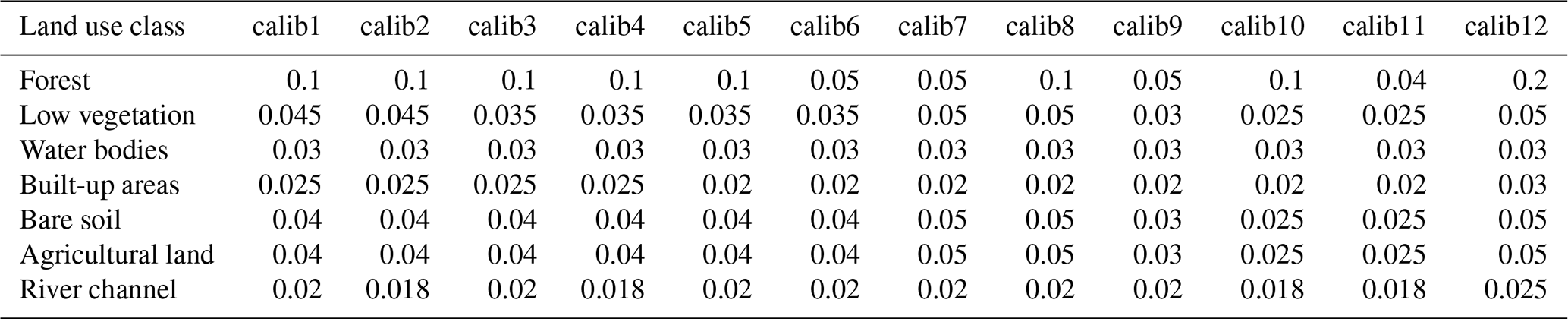
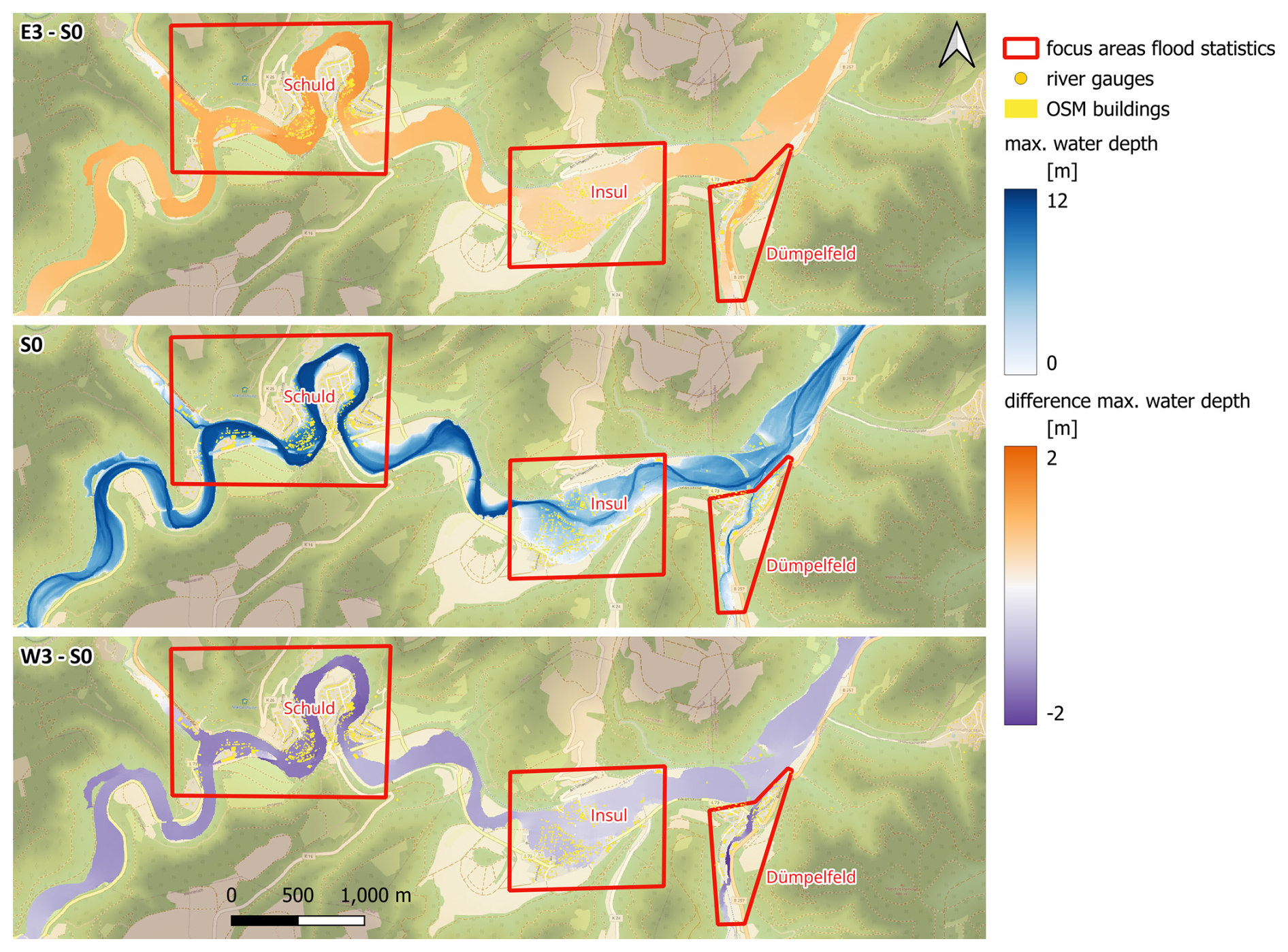
Figure A1 Inundated area and maximum water depths in the focus areas of Schuld, Insul, and Dümpelfeld for the reference scenario S0 as well as differences between E3 and S0 (E3–S0) and between W3 and S0 (W3–S0) scenarios. © OpenStreetMap contributors 2024. Distributed under the Open Data Commons Open Database License (ODbL) v1.0.

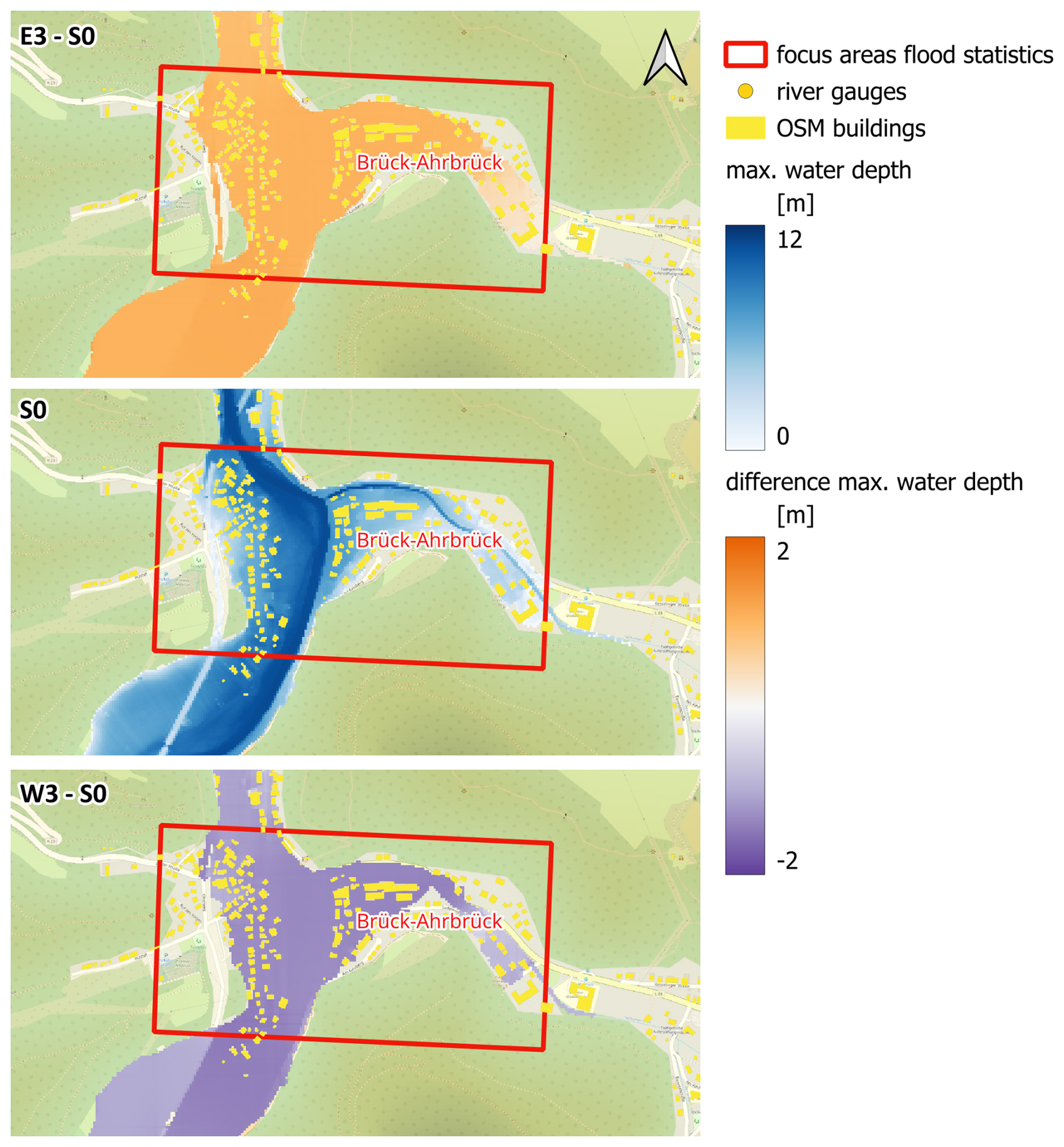
Figure A2 Inundated area and maximum water depths in the focus area of Brück-Ahrbrück for the reference scenario S0 as well as differences between E3 and S0 (E3–S0) and between W3 and S0 (W3–S0) scenarios. © OpenStreetMap contributors 2024. Distributed under the Open Data Commons Open Database License (ODbL) v1.0.

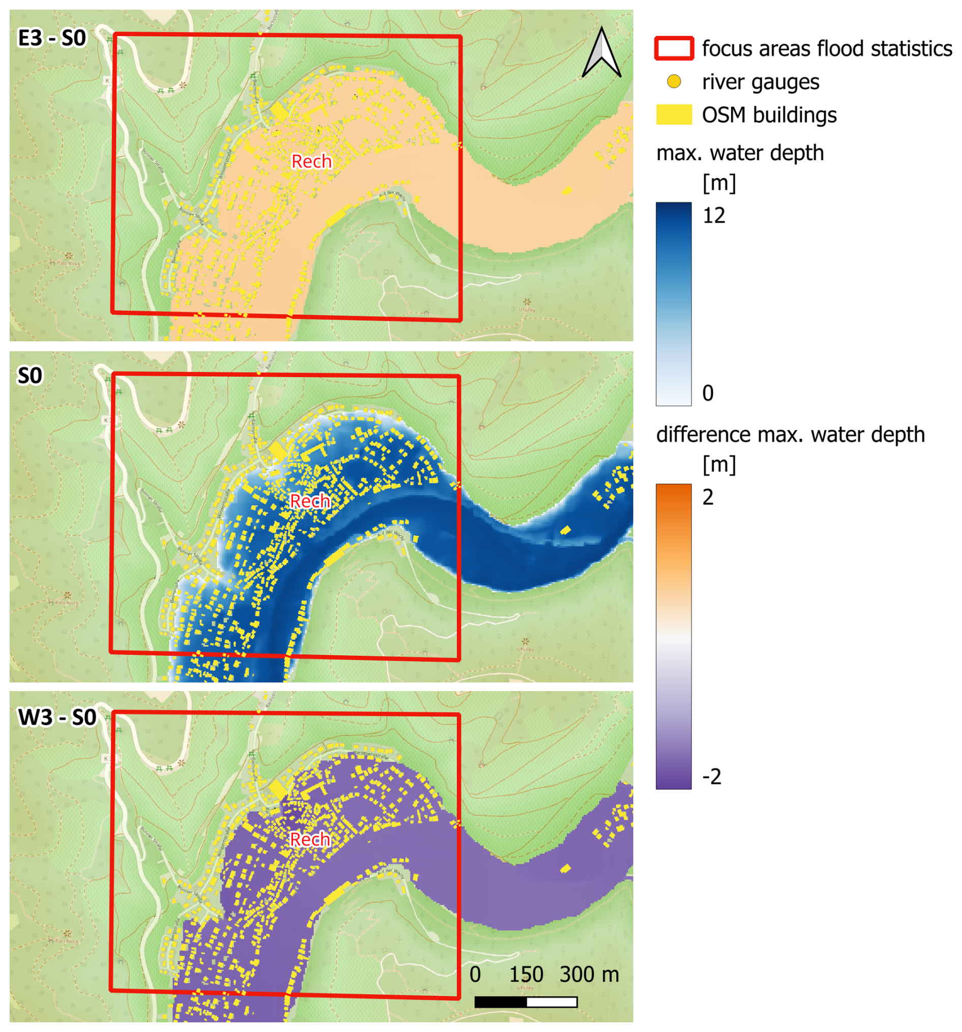
Figure A3 Inundated area and maximum water depths in the focus area of Rech for the reference scenario S0 as well as differences between E3 and S0 (E3–S0) and between W3 and S0 (W3–S0) scenarios. © OpenStreetMap contributors 2024. Distributed under the Open Data Commons Open Database License (ODbL) v1.0.

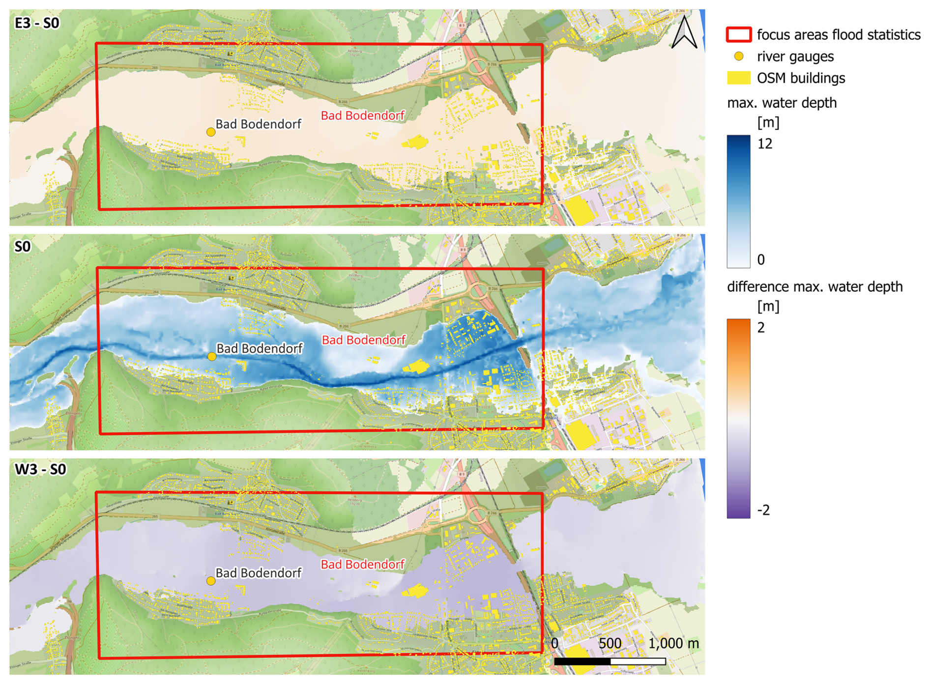
Figure A4 Inundated area and maximum water depths for the focus area of Bad Bodendorf for the reference scenario S0 as well as differences between E3 and S0 (E3–S0) and between W3 and S0 (W3–S0) scenarios. © OpenStreetMap contributors 2024. Distributed under the Open Data Commons Open Database License (ODbL) v1.0.