Development and validation of the terrain stability model for assessing landslide instability during heavy rain infiltration

Slope stability is a key topic, not only for engineers but also for politicians, due to the considerable monetary and human losses that landslides can cause every year. In fact, it is estimated that landslides have caused thousands of deaths and economic losses amounting to tens of billions of euros per year around the world. The geological stability of slopes is affected by several factors, such as climate, earthquakes, lithology and rock structures, among others. Climate is one of the main factors, especially when large amounts of rainwater are absorbed in short periods of time. Taking this issue into account, we developed an innovative analytical model using the limit equilibrium method supported by a geographic information system (GIS). This model is especially useful for predicting the risk of landslides in scenarios of heavy unpredictable rainfall. The model, hereafter named terrain stability (or TS) is a 2-D model, is programed in MATLAB and includes a steady-state hydrological term. Many variables measured in the field – topography, precipitation and type of soil – can be added, changed or updated using simple input parameters. To validate the model, we applied it to a real example – that of a landslide which resulted in human and material losses (collapse of a building) at Hundidero, La Viñuela (Málaga), Spain, in February 2010.

1 Introduction

Landslides, one of the natural disasters, have resulted in significant injury and loss to human life and damaged property and infrastructure throughout the world (Varnes, 1996; Parise and Jibson, 2000; Dai et al., 2002; Guha-Sapir et al., 2004; Crozier and Glade, 2005; Khan, 2005; Toya and Skidmore, 2007; Raghuvanshi et al., 2015; Girma et al., 2015). Normally, heavy rainfall, high relative relief and complex fragile geology with increased manmade activities have resulted in increased landslide (Gutiérrez-Martín, 2015). It is essential to identify, evaluate and delineate landslide hazard-prone areas for proper strategic planning and mitigation (Bisson et al., 2014). Therefore, to delineate landslide susceptible slopes over large areas, landslide hazard zonation (LHZ) techniques can be employed (Anbalagan, 1992; Guzzetti et al., 1999; Casagli et al., 2004; Fall et al., 2006).

Landslides are a result of intrinsic and external triggering factors. The intrinsic factors are mainly geological factors or the geometry of the slope (Hoek and Bray, 1981; Ayalew et al., 2004; Wang and Niu, 2009).

The external factor which generally triggers landslides is rainfall (Anderson and Howes, 1985; Collison et al., 2000; Dai and Lee, 2001). Several LHZ techniques have been developed in the past, and these can be broadly classified into three categories: expert evaluation, statistical methods and deterministic approaches (Wu and Sidle, 1995; Leroi, 1997; Guzzetti et al., 1999; Iverson, 2000; Crosta and Frattini, 2003; Casagli et al., 2004; Fall et al., 2006; Lu and Godt, 2008; Rossi et al., 2013; Raia et al., 2014; Canili et al., 2018; Zhang et al., 2018). Within these categories, we want to highlight the empirical models that are based on rainfall thresholds (Wilson and Jayko, 1997; Aleotti, 2004; Guzzetti et al., 2007; Martelloni et al., 2011). Each of these LHZ techniques has its own advantage and disadvantage owing to certain uncertainties on account of factors considered or methods by which factor data are derived (Carrara et al., 1995). Limit equilibrium types of analyses for assessing the stability of earth slopes have been in use in geotechnical engineering for many decades. The idea of discretizing a potential sliding mass into vertical slices was introduced in the 20th century. During the following few decades, Fellenius (1936) introduced the ordinary method of slices (Fellenius, 1936). In the mid-1950s Janbu and Bishop developed advances in the method (Janbu, 1954; Bishop, 1955). The advent of electronic computers in the 1960s made it possible to more readily handle the iterative procedures inherent in the method, which led to mathematically more rigorous formulations such as those developed by Morgenstern and Price and by Spencer (Morgenstern and Price, 1965; Spencer, 1967).

Until the 1980s, most stability analyses were performed by graphical methods or by using manual calculators. Nowadays, the quickest and most detailed analyses can be performed using any ordinary computer (Wilkinson et al., 2002). There are other types of software based on the modelling of the probability of occurrence of shallow landslides LHZ, in more extensive areas using geographic information system (GIS) technology and DEM (digital elevation model), as is the case of deterministic models like the software TRIGRS, SINMAP, R-SHALSTAB, GEOtop or GEOtop-FS, and r.slope.stability, among others (Montgomery and Dietrich, 1998; Pack et al., 2001; Rigon et al., 2006; Simoni et al., 2008; Baum et al., 2008; Mergili et al., 2014a, b; Michel et al., 2014; Reid et al., 2015; Alvioli and Baum, 2016; Tran et al., 2018). These are widely used models for calculating the time and location of the occurrence of shallow landslides caused by rainfall at the territorial level, some even in three dimensions, in order to obtain a probabilistic interpretation of the factor of safety. Currently other approaches and/or theoretical studies for landslide prediction are used (for triggering and/or propagation; Martelloni and Bagnoli, 2014; Martelloni et al., 2017). One of the achievements of the presented study is to discretize the potential slip mass in the critical profile of the slope, once unstable areas have been detected through the LHZ (landslide hazard zonation) programs. The terrain stability (TS) calculation tool is not limited to shallow landslides and debris flows but allows analysis of deep and rotational landslides, which other models often do not account for. We use the hydrological variable r_u of Spencer in our algorithm to consider the infiltration of rainfall in the calculation of stability of the considered slope.

Limit equilibrium types of analyses for assessing the stability of earth slopes have been in use in geotechnical engineering for last years. Currently, the vast majority of stability analyses using this method of the equilibrium limit are performed with commercial software packages like SLIDE V5, SLOPE/W, Phase2, GEOSLOPE, GALENA, GSTABL7, GEO5 and GeoStudio, among others (González de Vallejo et al., 2002; Acharya et al., 2016a, b; Johari and Mousavi, 2018). Currently there are other slope stability models based on the theory of limit equilibrium that are still in analysis and testing, as is the case with the SSAP software package (Borselli, 2012), but in this case a general equilibrium method model is applied. Secondly, sometimes for commercial models, the introductions of parameters to perform calculations are not very interactive. For the stability analysis, different approaches can be used, such as the limit equilibrium methods (Cheng et al., 2007; Liu et al., 2015), the finite element method (Griffiths and Marquez, 2007; Tschuchnigg et al., 2015; Griffiths, 2015) and the dynamic method (Jia et al., 2008), among others. Limit equilibrium methods are well known, and their use is simple and quick. These methods allow us to analyse almost all types of landslides, such us translational, rotational, topple, creep and fall, among others (Zhou and Cheng, 2013). For the stability analysis, different approaches can be used, such as the limit equilibrium methods (Zhu et al., 2005; Cheng et al., 2007; Verruijt, 2010; Liu et al., 2015), the finite element method (Griffiths and Marquez, 2007; Tschuchnigg et al., 2015; Griffiths, 2015) and the dynamic method (Jia et al., 2008), among others (SSAP 2012, Slide V5, 2018). Also, limit equilibrium methods can be combined with probabilistic techniques (Stead et al., 2006) or with other models, like stability analysis of coastal erosion (Castedo et al., 2012). However, they are limited in general to 2-D planes and easy geometries. Numerical methods – finite element methods – give us the most detailed approach for analysing the stability conditions for the majority of evaluation cases, including complex geometries and 3-D cases. Nevertheless, they present some problems, such as their complexity, data introduction, the mesh size effect, and the time and resources they require (Ramos Vásquez, 2017).

The above-mentioned software packages provide useful tools for determining the stability through the F_s (safety of factor) and for giving the most probable breakage (shearing) surfaces. This technique is fast and allows the field or emergency engineer to make timely decisions. Although this methodology is only available in some current software (Slide V 5.0, STB 2010, GEOSLOPE) and is based on limit equilibrium methods, it is highly recommended because of its reliability for representing real conditions in the field (Chugh and Smart, 1981). This rain infiltration produces a substantial reduction of cohesion (a key soil parameter for stability) that cannot be reproduced by actual software, and then several real situations cannot be predicted.

Delft University of Technology has developed a well-known and free software program to analyse landslides, the STB 2010 (Verruijt, 2010). This program is based on a limit equilibrium technique, using a modified version of Bishop's method to calculate the F_s only for circular failures. It is a user-friendly tool, but it does not allow the calculation of water infiltration on a hillside. This is a critical point, as it is well known that rainfall infiltration is one of the main causes of landslides worldwide (Michel et al., 2015). Reviewing these issues, a new solution must be developed for cases where landslides are linked to heavy rainfall. In this study, we developed a new model and programed it using MATLAB. The primary result of this model was a stability index, namely the minimum F_s, based on the limit equilibrium technique, in this case Bishop's method. The model also provides a possible failure curve and surface area, including the infiltration effects, which can be used to coincide with analysis of the actual event as tested with field data. Topographical data can also be introduced into the model from the DEM in a GIS.

2 Terrain stability model development

In the model we developed, the TS model, we used the limit equilibrium technique for its versatility, calculation speed and accuracy. An analysis can be done studying the whole length of the breakage (shearing) zone or just small slices. Starting with the original method of slides developed by Fellenius (1936), some methods are more accurate and complex (Spencer, 1967; Morgenstern and Price, 1965) than others (Bishop, 1955; Janbú, 1954). Using Spencer's method (Spencer, 1967; Duncan and Wright, 1980; Sharma and Moudud, 1992) here would mean dividing our slope into small slices that must be computed together. This method is divided into two equations, one related to the balance of forces and the other to momentum. Spencer's method imposes equilibrium not only for the forces but also for the momentum on the surface of the rupture. If the forces for the entire soil mass are in equilibrium, the sum of the forces between each slice must also be equal to zero. Therefore, the sum of the horizontal forces between slices must be zero as well as the sum of the vertical ones (Eqs. 1 and 2):

$$\begin{array}{}\text{(1)}& {\displaystyle }& {\displaystyle }\sum \left[Q\cos \mathit{\theta }\right]=\mathrm{0},\text{(2)}& {\displaystyle }& {\displaystyle }\sum \left[Q\sin \mathit{\theta }\right]=\mathrm{0}.\end{array}$$

In this equation, Q is the resultant of the pair of forces between slices, and θ is the angle of the resultant (Fig. 1). From this, it can be stated that the sum of the moments of the forces between slices around the critical rotation centre is zero, conformed to Eq. (3):

$$\begin{array}{}\text{(3)}& {\displaystyle }{\displaystyle }\sum \left[QR\cos \right(\mathit{\alpha }-\mathit{\theta })=\mathrm{0}].\end{array}$$

When the R is the radius of the curvature, α is the angle of the slope referred to each slice. This takes into account that the sliding surface is considered circular, so the radius of the curvature is constant.

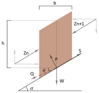
Figure 1 Representation of the forces acting on a slice, considered in Spencer's method (Spencer, 1967). W is the external vertical loads; Zn and Zn + 1 are the forces acting on the left- and right-hand side of each slice, respectively, with their horizontal and vertical components. P and S are the normal and tangential forces at the base of the slice; α is the angle of the slope referred to each slice, b is the slice width and h is the mean height of slice (if the height is not constant).

These equations must be solved to get the F_s and tilt angles of the forces among the slices (θ). To solve these equations, an iterative method is required until a limiting error is reached. Once F_s and θ are calculated, the remaining forces are also obtained for each slice. Spencer's method is considered to be very accurate and suitable for almost all kinds of slope geometries and may be the most complete equilibrium procedure. It may also be the easiest method for obtaining the F_s (Duncan and Wright, 2005). Depending on the type of slope analysed, this model is able to establish the failure curve following the typical rotational circle, among other uses (Verruijt, 2010).

The F_s, classically defined as a ratio of stabilizing and destabilizing forces, determines the stability of a slope as follows:

$$\begin{array}{}\text{(4)}& {\displaystyle }{\displaystyle }{F}_{\mathrm{S}}={\displaystyle \frac{\sum (\mathrm{Forces}\mathrm{standing}\mathrm{against}/\mathrm{oppose}\mathrm{sliding})}{\sum \left(\mathrm{Forces}\mathrm{that}\mathrm{induce}\mathrm{sliding}t\right)}}.\end{array}$$

According to limit equilibrium methods, the two equilibrium conditions (forces and moments) must be satisfied. Taking into account these elements, the F_s is then obtained from the following expression (Spencer, 1967):

$$\begin{array}{}\text{(5)}& {\displaystyle }{\displaystyle }{F}_{\mathrm{s}}={\displaystyle \frac{\mathrm{1}}{\sum W\sin \mathit{\alpha }}}\sum [c^{\prime }b\sec \mathit{\alpha }+\tan {\mathit{\varphi }}^{\prime }(W\cos \mathit{\alpha }-ub\sec \mathit{\alpha }\left)\right],\end{array}$$

where ϕ^′ is the friction angle at the fracture surface, u is the pore pressure at the fracture zone, c^′ is the soil cohesion, α is the angle at the base of the slice, W is the external vertical forces and b is the width of the slice. According to Eqs. (4) and (5), the slope can be considered unstable if its value of the safety factor F_s is lower than 1 or stable if it is equal to or higher than 1. It should be noted that, when applying the factor in the engineering and architecture fields, the limiting value tends to be higher than 1, with common values being 1.2 or even up to 1.5 (Burbano et al., 2009) and security coefficients that include the European technical regulations, specifically the technical regulations of Spanish application (Table 2.1 of the DB-C of the CTE, or technical code of the building), among others. This is just a confidence measure for your calculations. The F_s can also be defined as the ratio between the shear strength (τ), based on the cohesion and the angle of friction values, and the shear stress, based on the cohesion and the internal friction angle required to maintain the equilibrium (τ_mb).

As mentioned, the minimum F_s for considering a slope stable is equal to 1. However, several authors (Yong et al., 1977; Van Westen and Terlien, 1996) suggest that the angle of a slope would have to be defined by a value of the F_s superior to the unity to take into account the exogenous factors of the slope. Following Jiménez Salas (1981), a value of F_S≥1.3 can be considered stable by most standards.

To analyse the slope using Spencer's method, a set of equations must be solved to satisfy the forces and momentum equilibrium and to obtain the F_s. The values of F_s and θ are the unknowns that must be solved. Some authors suggest that the variation in θ can be arbitrary (Morgenstern and Price, 1965), although the effect of these variations in the final value of F_s is minimal. The variation in the angle depends on the soil's ability to withstand only a small intensity of the shear stress.

With that being said, if we assume that the forces between slices are parallel (in other words, that θ is constant), Eqs. (1) and (2) become the same, resulting in

$$\begin{array}{}\text{(6)}& {\displaystyle }{\displaystyle }\sum Q=\mathrm{0}.\end{array}$$

The assumption that the forces between slices are parallel gives optimal results for the calculation of the critical safety coefficients in Eq. (5) (Spencer, 1967). To solve these equations, we used the FSOLVE function of the MATLAB software, giving an initial F_s and angle. The FSOLVE function is a tool inside the optimization toolbox from MATLAB that solves systems of non-linear equations. When using this tool, an initial value must be provided to start the calculation.

When solving the normal and parallel forces at the base of the slice of the five acting forces, we obtain (Q), resulting from the forces between slices:

$$\begin{array}{}\text{(7)}& {\displaystyle }{\displaystyle }Q={\displaystyle \frac{\frac{c^{\prime }b}{F}\sec \mathit{\alpha }+\frac{\tan {\mathit{\varphi }}^{\prime }}{F}\left(W\cos \mathit{\alpha }-ub\sec \mathit{\alpha }\right)-W\sin \mathit{\alpha }}{\cos (\mathit{\alpha }-\mathit{\theta })\left[\mathrm{1}+\frac{\tan {\mathit{\varphi }}^{\prime }}{F}\tan (\mathit{\alpha }-\mathit{\theta })\right]}}.\end{array}$$

In this expression, u is the pore pressure (permanent interstitial pressure) at the base of the slice and the weight of the slice is determined by W. If we assume that the soil is uniform and its density (γ) is also uniform, the weight of a slice of height h and width b can be written as follows:

$$\begin{array}{}\text{(8)}& {\displaystyle }{\displaystyle }W=\mathit{\gamma }bh.\end{array}$$

The application of a homogeneous pore-pressure distribution (permanent interstitial pressure) has been included in the model (Bishop and Morgenstern, 1960). In this case, the permanent interstitial pressure on the base of the slice was determined by the following expression:

$$\begin{array}{}\text{(9)}& {\displaystyle }{\displaystyle }u=r_u\mathit{\gamma }h.\end{array}$$

In this expression, u is the pore pressure (permanent interstitial pressure) at the base of the slice, γ is the density of soil, h is the mean height of slice (if the height is not constant) and the weight of it affects the W evaluation.

The pore pressure will be hydrostatic, defined by the following: $u={\mathit{\gamma }}_w(h-h_w)$, where γ_w is the saturated density of soil, and h and h_w are the difference between saturated and dry height. The calculation of the infiltration factor is calculated with the following equation:

$$\begin{array}{}\text{(10)}& {\displaystyle }{\displaystyle }{r}_u={\displaystyle \frac{u}{\mathit{\gamma }h}}.\end{array}$$

The factor r_u is a coefficient of pore pressure (interstitial pressure coefficient), which determines the rain infiltration factor on the slopes. It is well known that the water that infiltrates the soil may produce a modification of the pore pressure, affecting its resistant capacity. This factor may vary from 0 (dry conditions) to 0.5 (saturated conditions). In the article of Spencer (Spencer, 1967), assuming a homogeneous pore-pressure distribution as proposed by Bishop and Morgenstern (1960), the mean pore pressure on the base of the slice can be written like Eq. (7).

This equation is used in our proposed model for calculating the safety factor (substituting the expression of u in Eq. 5).

3 Terrain stability (TS) algorithm and tests

Figure 2 shows the results of applying the terrain stability model to an irregular slope, including the initial and final points of the first failure circle (shown in yellow). This circle corresponds with the initial value introduced by the user into the FSOLVE function. The points of the slope are extracted from a DEM model in ArcGIS 10 (Glennon et al., 2008). The slope height is equal to 15 m, and the soil is considered to be uniform with the following nominal properties: γ=19 500 N m⁻³, φ=22^∘, c=15 000 N m⁻² and u=0 N m⁻². For the application example of our algorithm in this section, we have used geotechnical data of a cohesive soil of the flysch type of Gibraltar (González de Vallejo et al., 2002).

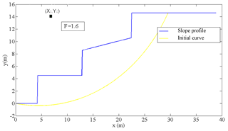
Figure 2 Idealized cross section of a slope. In this example, the centre coordinates are equal to x_c=7 m, y_c=14 m, and the lower cut has the slope coordinates (P1 point) equal to x_t=0 m and t=0 m, data that the user introduces.

The code works as follows: the initial circular failure curve is plotted using the FPLOT tool, as shown in Fig. 2 (yellow line). In this example, the centre coordinates are equal to x_c=7 m, y_c=14 m, and the lower cut has slope coordinates (P1 point) equal to x_t=0 m, y_t=0 m. The F_s obtained was 1.6, which is, in principle, a stable slope. It must be taken into account that the mass susceptible to sliding must be divided into a sufficient number of slices. This value is entered into our code through the parameter N. In the application example of our algorithm, the sliding mass was divided into N=500 slices; this value of N is entered into the code by the user, who decides the value of that parameter. The greater the number of slices in which we divide the sliding mass, the more accurate the calculation will be. For the N=500 slice, we consider it to be a balanced value for an optimal calculation, which relates two fundamental parameters (computer calculation capacity and capacity accuracy).

The next step is to apply Spencer's method to the different breakage surfaces until the curve with the lowest F_s is found, and that will be the critical surface susceptible to a circular slip. To determine the minimal F_s using this model, the algorithm calculates the displacement of the lower cut-off point of the critical slip from the slope as well as the position of the centre of rotation of the critical failure curve. In addition, the user must enter a series of possible circular faults. Then, the user introduces the following constraints into the program: the initial or lower point of the failure curve (P₁) in its intersection point with the slope, which may or may not match the origin of the slope analysed. Another restriction is the centre of the failure circle (X_c, Y_c), which should initially cut the slope, i.e. the breaking curve must be within the feasible sliding region. With these data, the program automatically draws a first curve, in this case the yellow line in Fig. 3, and calculates the safety coefficient F_s for that initial curve.

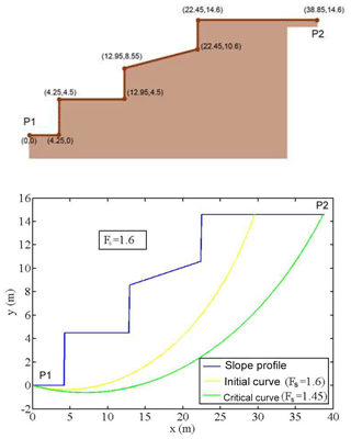
Figure 3 Results following the application of the software showing the slope profile and surface damage. The F_s and the clearest proof of circular failure are also provided (see the yellow line). P1 coordinates are (0, 0), and P2 coordinates are (38.85, 14.6) in metres.

On the basis of this first curve (yellow line in Fig. 2), the program enforces new restrictions:

• The curve passes through the origin of slope $P_{\mathrm{1}}=(\mathrm{0},\mathrm{0})$.

• The centre of the possible circles of critical breakage is inside the rectangular box defined as ($x_{\mathrm{box}\min .}<x_{\mathrm{c}}<x_{\mathrm{box}\max .}$; $y_{\mathrm{c}\mathrm{box}\min .}<y_{\mathrm{c}}<y_{\mathrm{box}\max }$). Note that the coordinates are entered with the 2-D expression (X, Y).

Both coordinates of the rotation centre position are free and can change for every circle. From the initial failure curve, characterized by the point x=(x_c, y_c), the MATLAB “fmincon” function is used to obtain a new critical point ($x_{\mathrm{c}}^{*}$, $y_{\mathrm{c}}^{*}$), where the F_s from the breakage curve is the minimum provided by fmincon. In this example, starting from the initial curve (yellow curve) with point $x=(\mathrm{7},\mathrm{14})$, the TS model provides a new point $x^{*}=(\mathrm{4.4910},\mathrm{28.1091},\mathrm{0})$ with a new F_s, F_S=1.45. In this case, the new search has been carried out with the following restrictions in the rectangular box, such as 2 m < x_c < 8 m and 16 m < y_c < 40 m. These restrictions are imposed in order to determine the critical circle. With all these restrictions, and because of the first calculated curve (the yellow curve), the developed model calculates the critical curve among the number of curves selected by the user (500 in this case), as well as the failure circle centre, by applying the fmincon (MATLAB function). This defines the curve with minimum F_s (F_min) as the value of F_s (see green curve in Fig. 3). When solving this problem, a critical selection is the lower cut-off point of the slope. According to different authors, such as Verruijt (2010) and Castedo et al. (2012), the selected point is the same as the P₁ point.

To complete the second phase in the TS model operation, the effect of rain infiltration must be introduced by the coefficient of the pore-pressure factor r_u. In this example, the infiltration factor was introduced at the base of each slice to account for the infiltration and pore pressure at the base of the break surface of the slope. If r_u increases, the cohesion of the soil mass of the slope decreases, directly affecting the reduction of the slope's F_s. The result is that a dry slope has F_S=1.45, but if including the r_u parameter equal to 0.3, the F_s decreases to a value of F_S=0.95, which means that an F_s is below the unity, so an unstable circular failure appears (see Fig. 4). Entering the infiltration factor, r_u, in Spencer's method to introduce the infiltration effects in slopes, the geotechnical cutting elements of the analysed soil are reduced, also reducing the values of the F_s, both for the initial yellow curve and the optimum green curve (Fig. 3). Note that the initial curve in the run shown in Fig. 4 is different from the one in Fig. 3, as it depends on the data introduced.

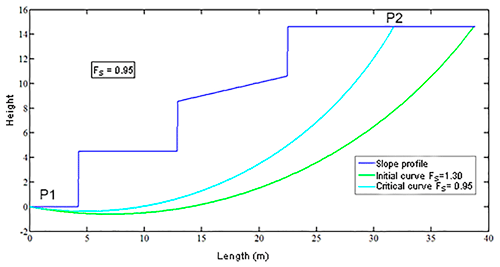
Figure 4 Outcome of the TS model after the introduction of the infiltration factor, producing an unstable circular failure (F_s=0.95).

We can determine that if this infiltration factor value is small enough, taking into account the safety coefficients, the design may still be adequate, but critical information was missing to calculate this parameter.

To clarify the procedure employed in the suggested algorithm, the flow chart (block diagrams) presented in Fig. 5 demonstrates the calculation and iteration process as implemented in our software.

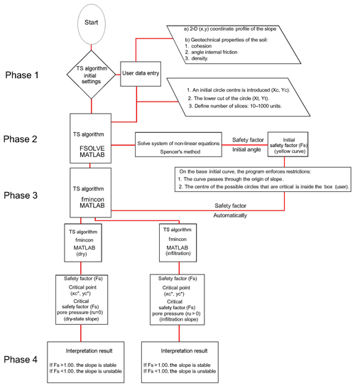
Figure 5 Sequential TS algorithm (block diagrams). Numbers in parentheses refer to numbers in the text.

Our algorithm (software) is more versatile compared to the STB 2010; the model developed here can analyse slope from right to left and vice versa, and the STB 2010 only allows the analysis from right to left. Other software programs, like the STB 2010, use a modified version of Bishop's method, a less accurate methodology than Spencer's method. A modified version of Bishop's method solves only the equilibrium in momentum, while the Spencer method also considers the equilibrium in forces.

Another improvement made by the TS code, in comparison with others, is that the use of Spencer's method allows us to analyse any type of slope and soil profile. In this procedure, we calculated the worst breaking curve by modifying the calculation points.

In the TS model, from the first slip rotational circle obtained in MATLAB, many circles were then calculated using the fmincon function, with some user restrictions. However, other models, like the STB 2010, require the definition of a quadrangular region (to look for the centres of rotational failures) and a point (namely five; see Fig. 9) to define the curve as where the failure must pass. Also, the number of circles that the STB 2010 model can analyse for their minimum value is limited to 100.

The TS model can detect relevant earth movements derived from rainfall infiltration, both translational and rotational types (Stead et al., 2006), such as those that usually occur in regions like India, the US, South America and the UK, among other places. The programs that do not contemplate this option will overestimate the F_s, potentially with great errors.

The TS model has an additional advantage: it also offers the opportunity to incorporate, in the same code, the stability analysis and the effect of the infiltration factor in the rainfall regime. This is a step forward from open-access programs, such as STB 2010, and also from alternative payment software, such as Slide.

4 Example of this application in the municipality of La Viñuela, Málaga, Spain

In 2010, La Viñuela, Málaga, (Spain) experienced torrential rainfall. The main consequence was a devastating landslide with serious personal and material losses, as shown in Fig. 6. The coordinates where this event occurred were in degrees (36.88371409801, −4.204982221126).

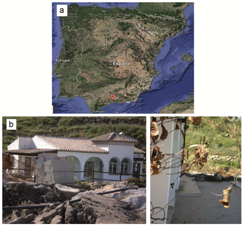
Figure 6 (a) Spanish map with the location of La Viñuela (Google Maps). (b) Real images taken by the authors at La Viñuela in 2010.

4.1 Geological and hydrological environment

The study area is located in the county of La Viñuela, specifically in the Hundidero village, which is located immediately north of the swamp of La Viñuela (El Hundiero) and south of the Baetic System mountain ranges (southern Iberian Peninsula).

According to the Cruden and Varnes' (1996) classification, the slide corresponds to a rotational slide-like complex movement because it was generated in two sequences at different speeds. This type of mechanism is characteristic of homogeneous cohesive soils, as was the one analysed here (Cornforth, 2005; Rahardjo et al., 2007; Lu and Godt, 2008).

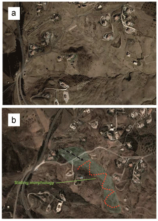
This event caused serious damage to different buildings. Regarding the damage caused, in the initial stretch of the slope (its head), a house was dragged and destroyed and another was seriously damaged. On the right bank of the mentioned house, another building was affected. In total, this event left a total of two buildings destroyed and one seriously compromised. Although 15 people lived in these houses, there were no fatalities. About 20 houses were to be constructed at the head of the slope; fortunately, the event happened before this construction. Figure 7 shows an aerial picture from 2006 before the disaster as well as the affected area and landslide in 2010.

Figure 7 (a) An aerial photograph from before the event (2006). (b) An aerial photograph taken after the landslide (2010).

4.2 Event features and geometry

For this example, we used data of IGN, the Spanish National Geographic Institute (http://centrodedescargas.cnig.es/CentroDescargas, last access: 11 December 2017), and a downloaded bitmap MTN25, which is a 1:25 000 topographic map in ETRS 89 coordinates and Universal Transverse Mercator (UTM) projection. The downloaded map is generated in a file by means of a geo-referenced digital rasterization (vector to raster conversion). Specifically, we downloaded page number 1039, which is the one corresponding to the landslide zone of the case study. Figure 8 shows the area of the case study.

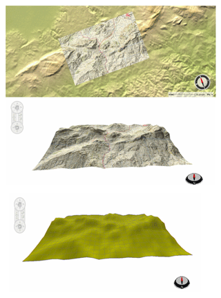
Figure 8 (a) Topographic map in a GIS map from page number 1039 of the IGN (Spanish National Geographic Institute).

From this map we obtained the topographic information to acquire all necessary profiles to study the landslide. Moreover, as our algorithm is a 2-D model, with this topographic map we study the critical curve of the slip in the most unfavourable profile of the landslide (Fig. 8).

It is well known that mass movements, such as landslides, are highly complex morphodynamic processes. We selected The Hundidero as our study area because it is prone to landslides. In order to analyse this case study using our model, we first calculated the initial displaced volume of the study area. According to the dimensions of the problem, the initial displaced volume was calculated, equivalent to the volume of half an ellipsoid (Varnes, 1978; Beyer, 1987; Cruden and Varnes, 1996) that has Vol = 1∕6π (width × length × depth). In our particular case, the width was equal to 70 m, the length was equal to 235 m, and the depth was equal to 5 m, making up a total volume of 4.364 m³ (Fig. 9). Taking an average of 33% elongation, as proposed by Nicoletti and Sorriso-Valvo (1991) and Cruden and Varnes (1996), we determined that the total material displaced in this landslide had an approximate volume of 5.804 m³. In this mass displacement, it is also necessary to consider material added by erosion and dragged from the initial mass displaced. In Fig. 7, the straight line indicates the first rotational movement, and the zigzag line shows the planar drag and glide after the first rotational movement. The green region is the total area displaced or affected by mass movement. After the first circular movement, the mass moved rapidly, associated with a continuous rise in incremental pore pressure and the rapid reduction of shear strength, without allowing pressure dissipation.

Figure 9 Characterization and longitudinal section of the rotational sliding (Geolen Engineering, 2010). The location of the dragged house is noted in red, which was analysed by the TS model.

The initial spit of land had an approximate size of 235 m in length by 70 m in width. Due to this initial displacement, there was a drag and a huge posterior planar displacement of about 550 m length, affecting a zone with several parcels of land and buildings. These sizes were confirmed using aerial photography and field data. The soil is basically composed of clays of variable thicknesses and of fine grain, with fluvial sediments and silty clay. The authors obtained these data by conducting a field survey as well as through the laboratory tests carried out by the laboratory Geolen S.A. (Geolen Engineering, 2010). From a geological and geotechnical point of view, according to a survey of those present as the laboratory extracted the materials, different lithological levels can be distinguished, as shown in Table 1.

Table 1 Lithology of the area affected by the failure, according to the laboratory tests of Geolen S.A. No groundwater level was detected.

The laboratory tests included a sieve analysis (following UNE 103 101) in three of the samples extracted from the field at depths of 1.80–2.00 m, of which 70.3 % were composed of clay and silt; according to this, the sample is classified as cohesive. The liquid limit and the plastic limit were determined in two of the samples (following UNE 103 103 and UNE 103 104, respectively), yielding liquid limit values of 57.5 % and 64.2 %, respectively, and a plasticity index of 37 %. According to the lab results, the material can be classified as high plasticity material with the potential of having a high water content. The landslide analysed began in February 2010, ending in March of that same year. However, based on the field inspection and the analysis of the rainfall series in the La Viñuela region in 2010 (see Fig. 10), it can be inferred that the main causes of the event were the following:

• the poor geomechanical parameters of the material that formed the affected hillside,

• the hydrometeorological conditions in the days preceding and days after the event, according to the histogram.

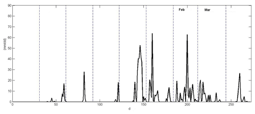
Figure 10 Rainfall histogram at La Viñuela from August 2009 to April 2010. Rainfall data have been provided by the Spanish Meteorological Agency (station of Viñuela).

Most of the landslides observed during these days occurred as a consequence of exceptionally intense rainfalls. The precipitation data were provided by the meteorological station of La Viñuela (Fig. 10). It can be observed that large amounts of precipitation fell during the months of December, January, February and March of 2010, with peaks being, at the most, 60 L m⁻² in a single day (January and February). In total, 890 L m⁻² fell in the 2009–2010 hydrological cycle, which ended at the end of April 2010. This is a key point in slope stability to consider when dealing with areas capable of having high infiltration rates.

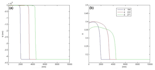
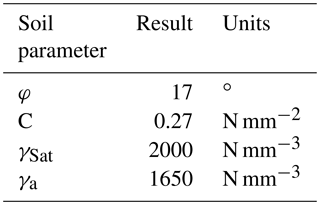
The rotational slide analysed had occurred between level 2 and level 3, when the water content reached that depth, as confirmed by the infiltration calculations in the terrain (see graphs in Fig. 9, reaching depths of up to 5 m). Two direct shear tests (consolidated and drained) were conducted in unaltered samples extracted from the boreholes at 3.00–3.60 and 4.00–4.60 m deep. The cut-off values of the soil are specified in Table 2. Those values were used in the developed software to obtain the safety coefficient and the theoretical failure curve.

Table 2 Summary chart of the characteristics of the soil analysed at the Geolen S.A. laboratory: φ is the angle of internal friction, c is the cohesion, γ_Sat is the saturated specific gravity and γ_a is the apparent specific gravity.

The dynamic and continuous tests were carried out by the Geolen S.A. laboratory with an automatic penetrometer of the ROLATEC ML-60-A type. The data obtained were transcribed by the number of strokes to advance the 20 cm tip, which is called the “penetration number” (N₂₀).

This test is included in the ISO 22476-2:2005 standard as a dynamic probing super heavy and consists of penetrating the ground with a conical tip of standard dimensions. The depth of the failed mass can be estimated as well as the theoretical failure curve for an increase in the soil consistency (see data in Table 3).

Table 3 Summary chart of the soil analysed at the Geolen S.A. laboratory. Bold values show, according to the data of the field penetrometers, the depth mobilized by the rotational sliding.

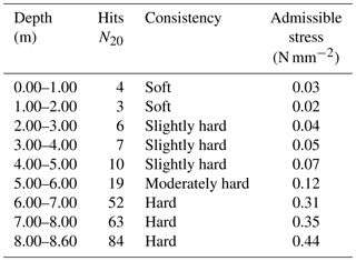
The change in the geomechanical response of the soil takes place at a depth of 4–5 m, according to the results of N₂₀ and US (samples without changes) taken along the analysed column. In this case, the sloped ground mass showed a characteristic striking relationship of a displaced terrain (Gonzalez de Vallejo et al., 2002). This differs from the underlying or unmoved terrain, which indicated a more consistent striking relationship that was taken within the area of the landslide behind the house drawn in accordance with the analysis of the hits N₂₀ from Table 3.

Figure 11 (a) Hydraulic potential. (b) Volumetric water content. Both have been plotted as a function of the depth (mm) at different times (d).

4.3 Input data

To analyse the topography of the critical section, we obtained the DEM data from the ArcGIS 10 software program (Environmental System Research, 2017), with a scale of 1:1000, through IGN raster maps, with adequate accuracy. These data were interpolated to a 2 m grid using a triangulated network interpolation methodology. Orthophotos proved to be very useful in locating the landslide with accuracy and to validate the field survey. The model developed here applies to failure in an initiation zone, in addition to predicting landslides, including those induced by the infiltration of critical rains.

To complete the input data, we plotted the hydraulic potential and the volumetric water content, as a function of depth in the ground for different time steps, using a previously developed infiltration model, as shown in Fig. 11 (Herrada et al., 2014). The figure shows the evolution of how the wetting front advances can be observed. These reached almost 5 m depth at the end of April 2010.

4.4 Analytical results

We applied the TS model using topographic data obtained from the ArcGIS 10 software program. We did so to obtain the degree of stability of the sliding land based on the angle of internal friction, the cohesion, the density and the angle of the slope we analysed. Figure 9 shows the analytical results from the real slope by studying and analysing the most unfavourable profile of the landslide studied. In addition we compared the results given by the developed TS model and the results given by STB 2010 model, using free surfaces in both cases. In our model the worst curve (shown in green) was calculated automatically from the initial curve (shown in blue), resulting in F_S=2.300, in the dry state (Fig. 12).

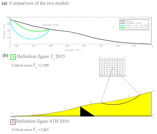
Figure 12 (a) TS model with a critical failure of F_S=2.300. (b) Results are from the STB 2010 model with an F_s of 2.063.

As can be noted, the failure curves are similar, and the safety coefficients F_s only differ by 0.237. In both cases, the results indicated are conservative estimates, resulting in a stable slope that was not realistic, as was the case in La Viñuela. In order to get the most unfavourable curve, which would match the analysis of the actual event, the pore coefficient must be introduced. At the first runs of the model, the r_u was equal to zero (dry soil in Fig. 9), but if this value is changed to r_u=0.35, the results are quite different (Fig. 13). The resulting failure was near the surface and the top cut with the slope found relatively near to the houses. Taking into account the infiltration of rainwater, the slope analysed in the TS model showed a value of F_S=0.98, in other words showing that it was unstable.

Figure 13 A new calculation including the pore coefficient r_u, showing the worst curve in green. The circles show the houses dragged by the landslide.

This calculation and the theoretical failure curve provided by our model was able to reproduce, in a realistic way, the landslide which occurred in La Viñuela. Our model found that the critical surface area that corresponded with the profile of the terrain was 12 927.45 m², which closely matches the real situation. In the STB 2010 program, it was 7825.35 m²; therefore, our prediction was more accurate.

As mentioned, the STB 2010 model does not allow stability calculations to apply to rainfall infiltration on a hillside. Hence, it is not capable of predicting a hillside's instability in a critical rainfall scenario, which was critical in the slope analysed. The STB 2010 model found that the hillside studied had an F_s of F_S=2.063; that means that it was a very stable slope. Consequently, our original algorithm TS model appears to be more efficient and accurate.

If we compare the results of the penetrometric tests (Table 3) and the laboratory tests (Geolen Engineering, 2010) summarized in the actual critical surface in the most unfavourable profile of landslide (Fig. 9) with those offered by our TS algorithm (Fig. 13) to which we apply the infiltration factor r_u=0.35 (high interstitial pressure), we can check the similarity between the two critical surfaces of the landslide.

A value of r_u=0.35 was introduced in the calculation, and the code gave us a value of the slope safety factor of F_s=0.95 (unstable); when in the dry state, the code calculated a safety factor of F_s=2.300 (stable). The calculation of the safety factor in the STB 2010 program that lacks the analysis of infiltration in the calculation offered a result of F_s=2.063 (stable).

Using the STB 2010 program, we would not have been able to previously detect the landslide of the case study of the paper, calculation that is not normally done in the stability calculations; with the calculation with our code we could have avoided the collapse of the building.

With these results, the terrain stability analysis performed using the developed model defines the slip-breaking curve that intuitively appears to be susceptible to failure fairly well, especially when heavy rains occur. For example, the landslides which occurred in the La Viñuela area could only have been predicted if the infiltration had been taken into account. Even then, it could not have been done with other available software programs, which were not able to consider it.

5 Conclusion

The terrain stability (TS) analysis defines the critical surface to landslides in 2-D of each profile of the analysed slope and the safety slip factor (F_s) fairly well. We developed this model due to the need for a useful tool to predict landslides, especially when heavy rains occur.

The TS model we developed uses Spencer's method, which is more precise than the modified Bishop method; this model is used by other software such as the case of the STB 2010, so it differs in the results it provides for the F_s. It also takes into account the factor of water infiltration due to critical rains, which other software programs do not consider. A failure surface can be determined by constraints using the MATLAB function fmincon. The data needed to run the model include soil and climate properties that may vary in space and time. The exit indices of the analysis (F_s) should be interpreted in terms of relative risk. The methods implemented in the TS model are based on data structures, which are based on the data entry of the elevation model (DEM), so we obtain a topographic map, a key element in obtaining the topographic profile to be studied with our algorithm.

In the case study analysed, the slope was initially stable and was determined by the analysis performed with the STB 2010 model. However, the slope became unstable due to the heavy rains of that hydrological period, which called for the application of the pore-pressure coefficient r_u. For analysing cases of heavy rain, this model is a powerful tool for determining slope stability. In addition, thanks to the great versatility of this model, it is applicable to any analysis in other parts of the world, based on the methods of limit equilibrium (Spencer, 1967). The TS model can also be used in combination with GIS software, SINMAP, the TRIGRS model and aerial photographic analysis, and mapping techniques, or even as a part of other models like the coastal recession models (Castedo et al., 2012).