Tsunami run-up estimation based on a hybrid numerical flume and a parameterization of real topobathymetric profiles

Tsunami run-up is a key value to determine when calculating and assessing the tsunami hazard in a tsunami-prone area. Run-up can be accurately calculated by means of numerical models, but these models require high-resolution topobathymetric data, which are not always available, and long computational times. These drawbacks restrict the application of these models to the assessment of small areas. As an alternative method, to address large areas empirical formulae are commonly applied to estimate run-up. These formulae are based on numerical or physical experiments on idealized geometries. In this paper, a new methodology is presented to calculate tsunami hazard at large scales. This methodology determines the tsunami flooding by using a coupled model that combines a nonlinear shallow water model (2D-H) and a volume-of-fluid model (RANS 2D-V) and applies the optimal numerical models in each phase of the tsunami generation–propagation–inundation process. The hybrid model has been widely applied to build a tsunami run-up database (TRD). The aim of this database is to form an interpolation domain with which to estimate the tsunami run-up of new scenarios without running a numerical simulation. The TRD was generated by simulating the propagation of parameterized tsunami waves on real non-scaled profiles. A database and hybrid numerical model were validated using real and synthetic scenarios. The new methodology provides feasible estimations of the tsunami run-up; engineers and scientists can use this methodology to address tsunami hazard at large scales.

1 Introduction

Recent tragic tsunami events, like those that occurred in the Indian Ocean in 2004, in Chile in 2010 and in Japan in 2011 have exposed the need for further work to develop and apply tsunami risk reduction measures. The adequate evaluation of tsunami hazard in tsunami-prone areas is the first step in a proper risk evaluation (UNESCO-IOC, 2009). Determination of the tsunami hazard focuses on the estimation of the area that would be flooded during a tsunami and on the calculation of the variables or parameters that define the phenomenon in that area, e.g., wave amplitude, current depth, tsunami travel time etc. Among these parameters, maximum run-up provides the elevation to which water from a tsunami wave will rise during its flooding process. Therefore, run-up is a key parameter that must be adequately determined when assessing the inundation of affected areas.

Figure 1 Distribution of sample profiles.

When tsunami hazard is addressed at a local scale (tens of kilometers or one coastal city), the optimal methodology to calculate the flooding and run-up is typically the application of validated deterministic numerical models (Álvarez-Gómez et al., 2013; Titov et al., 2011; Wang, 2009). These models allow reproduction of the three main tsunami processes: generation, propagation and inundation. To address these processes and to properly estimate the flooded area, high-resolution topography–bathymetry data of the study area are required, as well as the focal parameters that define the tsunamigenic mechanism. Nevertheless, the application of tsunami numerical models has some limitations and uncertainties (Park et al., 2015; Selva et al., 2016). First, their use requires a high computational cost and expert modelers. Second, the necessary high-resolution data to properly study the hazard in local areas are not always available. In addition, the correct definition of the tsunamigenic mechanisms, e.g., the parameters of the focal mechanism, contains uncertainties in itself. Finally, even though models are evolving to reduce uncertainties, there is still ongoing work on several aspects, such as wave transformation near the coast, interaction of waves with coastal structures, and accurate incorporation of bottom friction.

On the other hand, in large-scale studies (hundreds of kilometers or the coast of a whole country), the drawbacks of numerical models are more evident, and the lack of continuous high-resolution topobathymetry and the elevated computational cost foster the use of other approaches. An alternative methodology to estimate the tsunami run-up and, consequently, the flooded area, includes the application of run-up analytical or empirical formulae. In these cases, numerical models, despite the lower resolution of bathymetry, adequately calculate the tsunami wave characteristics offshore and can then be used as input for the formulae. Afterwards, by applying this method to several topobathymetric profiles along the coast, the total flooded area due to tsunami action can be estimated.

The calculation and analysis of run-up was initially approached by Carrier and Greenspan (1958). They found the exact solution for the nonlinear shallow water equations for a sloping beach with non-breaking regular waves. Keller and Keller (1964) derived an analytical solution for linear shallow water waves at a constant depth moving up a constant slope beach. This geometry has become the canonical problem. Synolakis (1987) extended Carrier and Greenspan's result to this problem by joining Carrier and Greenspan's and Keller and Keller's solutions to provide a closed-form solution for solitary wave run-up. Synolakis' results are remarkable, as solitary waves have been widely used to model tsunamis, numerically and physically. Li and Raichlen (2001) revisited Synolakis's results to determine the importance of a higher order correction to the analytical approach. Later, Madsen et al. (2008) demonstrated that solitary waves do not represent the large scale of a tsunami, and Chan and Liu (2012) confirmed this affirmation. Madsen and Schäffer (2010) found closed-form solutions for the run-up of waves of several shapes; their solutions included other parameters, such as the period, achieving more realistic results. Finally, Fuentes et al. (2015) studied the run-up on multilinear sloping beaches.

In addition, run-up has been commonly linked with the Iribarren number (Iribarren and Nogales, 1949), also called the surf similarity parameter (Battjes, 1974). Hunt (1959) joined this parameter with the non-dimensional run-up of regular waves. Kobayashi and Karjadi (1994) combined physical and numerical simulations to derive an equation to calculate run-up, using the ratio between the run-up and the wave amplitude and its relationship with the surf-similarity parameter. Fuhrman and Madsen (2008) demonstrated that the relationship between surf-similarity and solitary waves was similar to the that between surf-similarity and period waves.

More recently, several authors have focused their work on calculating tsunami run-up by developing new models with other approaches. Sepúlveda and Liu (2016) presented expressions for the calculation of the run-up based on the parameters that defined the focal mechanism of the tsunamigenic seism. Riquelme et al. (2015) derived simple solutions to estimate run-up on nearfield tsunamis by extending Synolakis solution (Synolakis, 1987) and Park et al. (2015) defined the run-up for compound slopes, based on the work of Madsen and Schäffer (2010) and numerical simulations of tsunami waves on two-slope topobathymetric profiles.

However, the application of these equations and formulae is not always evident, and each approach considers different inputs. Moreover, the parameterization presented by Carrier and Greenspan (1958), extended by Synolakis (1987) and modified by Park et al. (2015), is based on theoretical bathymetric profiles. It does not explicitly consider real profiles or the geometry of the whole area, from the tsunami generation zone to the flooded area. Furthermore, the numerical models that do consider the natural geometry of the bathymetric profiles adequately predict propagation, but they cannot accurately solve the flooding calculation, in addition to the other exposed drawbacks.

Complementing these methodologies, this work presents an alternative methodology to calculate tsunami flooding at large scales and is focused on assessing the run-up. The methodology is then applied to further develop a database from which the tsunami run-up of new scenarios can be interpolated.

The main component of the methodology is a numerical flume where the simulations are run. This flume was developed by combining a nonlinear shallow-water-equations model and a Navier–Stokes volume-of-fluid model to create a hybrid model that applies the optimal numerical model in each area of the flume. Time series of tsunami waves and topobathymetric profiles are used as input to calculate the run-up.

This hybrid model has been applied to further develop a database from which the run-up of new tsunami scenarios can be interpolated. This database contains an adequate representation of natural bathymetric profiles worldwide and the variability in tsunami wave shapes, allowing calculation of the tsunami run-up of new scenarios by interpolation without running a numerical simulation.

The aim of this methodology is to help specialists to further develop tsunami hazard maps at large scales, where the application of numerical models is not computationally affordable and high-resolution data are not available. This method can be used to quickly estimate the run-up in tsunami-prone areas or accurately estimate the flooded area for new tsunami scenarios.

The paper is structured as follows: Sect. 2 describes the developed methodology, including the parameterization of realistic bathymetric profiles and tsunami wave shapes and the construction of the numerical flume. In Sect. 3, the application of the methodology to calculate the tsunami run-up database is discussed, together with a sensitivity analysis of the influence of each parameter on the final value of the run-up. Section 4 includes details of the tool that has been developed in order to use the database to calculate new tsunami event run-ups. Section 5 presents the validation of the methodology with real and numerical scenarios. Finally, Sect. 6 discusses the conclusions drawn from this work.

Figure 2 Scheme of the parameterized profiles, based on real profiles analyses. The profiles are defined by three angles (tanβ₁, tanβ₂ and tanβ₃) and two depths (d₁and d₂).

2 Tsunami run-up hybrid model methodology

The run-up calculation methodology presented in this paper consists of the numerical simulation of tsunami waves along real non-scaled bathymetric profiles that were previously parameterized.

To carry out these simulations, a numerical flume was designed; this flume is formed by the coupling of two numerical models.

The Cornell Multi-grid Coupled Tsunami Model (COMCOT, Wang, 2009) solves the nonlinear shallow water equations (NLSWE) using a leap-frog finite differences scheme on a 2-D horizontal domain. In addition, the IH2VOF model (Lara et al., 2006) solves volume-averaged Reynolds-averaged Navier–Stokes (VARANS) equations based on the decomposition of the velocity and pressure fields into mean and turbulent components using a k-ε turbulent model on a 2-D vertical domain. More specifically, IH2VOF uses a log-law distribution of the mean tangential velocity in the turbulent boundary layer near the solid boundary. The values of k (turbulent kinetic energy) and ε (dissipation rate of turbulent kinetic energy) can be expressed as functions of the distance y from the solid boundary and the mean tangential velocity outside the viscous sublayer. (Garcia et al., 2004; Hsu et al., 2002; Lara et al., 2006; Lin and Liu, 1998; Pengzhi Lin and L.-F. Liu, 1999). On the free surface, the zero gradient boundary conditions for both k and ε are based on the assumption of no turbulence exchange between water and air. The equations of the k-ε turbulence transport model are as follows:

$$\begin{array}{}\text{(1)}& \text{free surface: no flux condition}:{\displaystyle \frac{\partial k}{\partial n}}={\displaystyle \frac{\partial \mathit{\epsilon }}{\partial n}}=\mathrm{0},\end{array}$$

$$\begin{array}{ll}{\displaystyle }\text{solid wall:}& {\displaystyle }\text{log-law turbulent boundary layer for}\\ \text{(2)}& {\displaystyle }& {\displaystyle }\text{smooth surface}{\displaystyle \frac{\overrightarrow{u_{\mathrm{n}}}}{u_{\ast }}}={\displaystyle \frac{\mathrm{1}}{K}}\ln \left({\displaystyle \frac{E{u}_{\ast }y}{\mathit{\nu }}}\right),\end{array}$$

where n is the unit normal on the free surface, K is the von Karman constant, y is the distance from the solid domain and u_∗ is a friction velocity. A smooth wall function was used to simplify the application of the hybrid model. E is a constant that is equal to 9.0 for smooth wall.

COMCOT model is prepared to simulate the stages of tsunami propagation; meanwhile, IH2VOF model is specially designed to simulate the coastal processes and wave transformations present when the waves reach the coastal areas. IH2VOF model calculates the run-up by evaluating the water accumulated in each column of the grid, tracking the changes on each cell density.

In the flume, the strengths of both models are used to design a numerical space where tsunami waves are propagated, using COMCOT from the deep ocean (∼ 4 km depth) to the coast, where the capabilities of the IH2VOF model are applied to calculate the flooding. As a result, a hybrid model that adequately solves the tsunami processes in both deep and shallow waters was achieved.

Parameterized profiles and a tsunami wave time series dataset are used as input for the numerical flume. These inputs, the most relevant aspects of the numerical flume geometry and the coupling of the models are described below.

2.1 Bathymetric profile characterization

Worldwide bathymetric profiles were analyzed, with a focus on finding a parameterization that properly represents natural shapes.

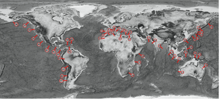
To cover the existing variability in the world bathymetry, a representative sample of 50 averaged profiles was obtained from tsunami-prone coastal areas and basins, namely, the Pacific Ocean, Indian Ocean, Mediterranean Sea and Caribbean Sea (Fig. 1). Topographic and bathymetric information was obtained from the General Bathymetric Chart of the Oceans (GEBCO, International Hydrographic Organization, 2014, with a cell size $\mathrm{\Delta }x={\mathrm{30}}^{\prime \prime }$), The European Marine Observation and Data Network (Bathymetry Consortium EMODnet, 2016) and the local bathymetry data that was available. The shape of these profiles was analyzed to perform an adequate parameterization.

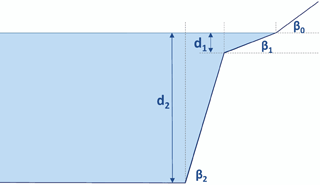
The propagation of a tsunami can affect thousands of kilometers; thus, the profiles must extend under both deep water and shallow water to capture tsunami generation to flooding. Considering this requirement, profiles were defined from inland (50 m height) to the deep ocean (∼ 4000 m depth). To avoid singularities, each defined profile is the average profile of a 10 km-wide coastal segment. Based on the bathymetric shapes observed in this selection, a representative and functional parameterization the profiles was tackled, using five parameters: three slopes (tan β₁, tan β₂ and tan β₃) and two depths (d₁ and d₂). Figure 2 shows the five-parameter geometry.

As an example, in Fig. 3, a selected profile from the Indonesian coast is shown, as well as its parameterized profile that was created by applying the five-parameter geometry. The parameters for each considered profile were fitted by using a least-squares method.

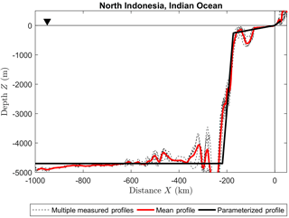
Figure 3 Sample of measured topobathymetric profiles on the Indonesian coast, as well as the mean and parameterized profiles. GEBCO was used as source for the topobathymetric data (Cell size $\mathrm{\Delta }x={\mathrm{30}}^{\prime \prime }$).

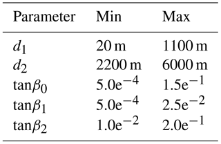
The maximum and minimum values of the five parameters are shown in Table 1. These values cover a wide range of the profiles that can be found in nature. Despite not including all the existing geometries, the maximum and minimum values certainly provide enough information to characterize the topobathymetric profiles.

Table 1 Maximum and minimum values of the profile parameters.

2.2 Initial tsunami wave characterization

The numerical flume described in detail in the next subsection requires not only the topo-bathymetric profile characterization but also the characteristics of the tsunami waves as input. To use these data as input for the hybrid model, a time series of the offshore wave amplitude must be provided. These time series could be obtained from either records of real tsunamis, e.g., from DART buoys, or from the results of numerical model tsunami propagation. In this case, COMCOT (Wang, 2009) was adopted. This model calculates all stages of tsunami modeling (generation, propagation and coastal flooding).

The generation of the tsunamis in COMCOT is approached via elastic finite fault plane theory, using the so-called Okada model (Okada, 1985). This model assumes an idealized rectangular fault plane as a representation of two colliding tectonic plates. The Okada model requires seven focal mechanism parameters as input to calculate the initial deformation of the water surface due to the earthquake. These parameters are the focal depth (h_focal), rupture length (L) and width (W) of the fault plane, dislocation (D), strike direction (θ), dip angle (δ) and slip (rake) angle (λ). An instantaneous tsunami generation with a constant distribution of the slip is assumed. A simulation of the numerical model provides the wave amplitude time series to be used as input for the hybrid model.

2.3 Numerical flume geometry

The dimensions of the numerical flume vary with the profile characteristics, adapting the domain for each simulation. The geometry of the flume is shown in Fig. 4. The total length L of the flume is split into two components: L_off is the submerged part of the profile and L_i is the inland part of the profile.

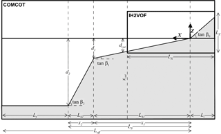
Figure 4 Numerical flume geometry, including the five parameters that define each profile (tan β₁, tan β₂, tan β₃, d₁ and d₂) and the general location of x_cut, where numerical models are coupled.

L is determined for each simulation according to the profile parameters (tanβ₁, tanβ₂, tanβ₃, d₁ and d₂), and the tsunami wave length is $\mathit{\lambda }=T\cdot \sqrt{g\cdot h}$, where T is wave period and g is the gravitational acceleration:

$$\begin{array}{}\text{(3)}& L=L_{\mathrm{i}}+L_{\mathrm{off}},\end{array}$$

$$\begin{array}{}\text{(4)}& L_{\mathrm{i}}={\displaystyle \frac{\mathrm{50}}{\tan {\mathit{\beta }}_{\mathrm{0}}}},\end{array}$$

$$\begin{array}{}\text{(5)}& L_{\mathrm{off}}=L_f+x_{\mathrm{2}}+x_{\mathrm{1}},\end{array}$$

$$\begin{array}{}\text{(6)}& L_f=⌈{\displaystyle \frac{\mathrm{1.2}\cdot \mathit{\lambda }}{\mathrm{10}\cdot \mathrm{\Delta }x}}⌉\cdot \mathrm{\Delta }x\end{array}$$

$$\begin{array}{}\text{(7)}& x_{\mathrm{2}}={\displaystyle \frac{d_{\mathrm{1}}}{\tan {\mathit{\beta }}_{\mathrm{1}}}}+{\displaystyle \frac{d_{\mathrm{2}}-d_{\mathrm{1}}}{\tan {\mathit{\beta }}_{\mathrm{2}}}},\end{array}$$

where Δx is the resolution (cell size) of the simulation with the COMCOT numerical model, as described in detail in the next section. In Eq. (4), Δx is in both denominator and numerator to round L_f to the order of Δx, by means of “ceiling brackets”.

The IH2VOF domain is located in the shallowest part of the profile, with a sufficient area of the inland domain to obtain an accurate measurement of run-up and an area as long as possible for the wave propagation.

The design of the domain of the RANS model followed several conditions. First, the maximum number of cells in X (horizontal dimension) was set at 5499 (n_x < 5499) in order to avoid too long computational times. Then, the ratio between the dimensions of the cell on each direction must be constant ($r=\mathrm{\Delta }x/\mathrm{\Delta }z=$ constant) and, in this case, a scale relation of r= 5 ∕ 1 was applied. Although this ratio may lead to a slightly premature breaking of the wave (Jacobsen et al., 2012) it limits the computational times relative to those achieved with smaller aspect ratios. Therefore, the maximum length covered with the RANS model was $L_x=n_x\cdot \mathrm{\Delta }x$, which led to IH2VOF grid lengths from 500 to 25 000 m. Finally, to avoid the false breaking of the wave, the Z (vertical dimension) of the IH2VOF model grid was discretized in a number of cells, satisfying the following expression:

$$\begin{array}{}\text{(8)}& \mathrm{\Delta }z=⌈{\displaystyle \frac{K\cdot H_{\mathrm{COMCOT}}}{N_{\mathrm{c}}\cdot \mathrm{0.05}}}⌉\cdot \mathrm{0.05},\end{array}$$

where K is a safety margin of the model K=1.08 and Δz, is defined in meters in the range (0.05 < Δz < 1). The wave height was discretized in N_c =10 cells to avoid false breaking. The effect of the ceiling brackets is “rounding to the lowest integer”. A constant cell height is assumed in the IH2VOF domain. Grids construction must follow literature validations (Torres et al., 2007, 2009; Lara et al., 2011) to set the cell dimensions, avoiding the case wherein first grid point falls out of the log layer.

2.4 Numerical models coupling

The coupling of the numerical models was focused on accurately locating the border position between the models, x_cut (see Fig. 4). This location is optimized in the domain of the IH2VOF model for every tsunami scenario, as that area is the most computationally demanding. For this optimization, two criteria were followed: (1) maximize the area of the IH2VOF domain and (2), simultaneously ensure that the flooding does not exceed the inland limit of the IH2VOF domain. In this sense, the number of cells of the IH2VOF model drives the generation of the grid. The position where the models are coupled, x_cut, is given by the value of L_x. In addition, since the flume is non-scaled, it was not possible to cover the whole domain with the RANS model due to computational restrictions (i.e., the generation–propagation and inundation areas cannot be calculated without assuming other limitations of scale). However, offshore generation and propagation is well solved by the NLSWE model, since non-linearities are less relevant in those processes. The NLSW model does not describe physical dispersion, which is important in the generation of some physical effects, like undular bores. These effects are described by IH2VOF, depending on the local steepness of the tsunami wave entering its domain.

Thus, to properly define the IH2VOF domain, it is necessary to know in advance a rough value of the run-up to fit the inland part of the grid L_i to each specific case. In this sense, the more accurate the rough estimate of the run-up is, the fewer inland cells are wasted (without flooding), meaning that the IH2VOF performance is optimized. Clearly, the complete run-up must be fully covered by this model domain, meaning that the vertical length of the onshore grid L_z must be adequate. To determine this horizontal length in advance, each simulation is precalculated with only COMCOT to obtain an approximation of the run-up of the considered tsunami scenario.

The transference of data between models occurs at x_cut. IH2VOF requires as input a time series of sea surface deformation and a velocity profile; hence, these data are obtained as an output of the COMCOT model. Nevertheless, in most cases, the tsunami wave length λ is considerably longer than the length of the IH2VOF grid L_x (λ > L_x). Therefore, before the entire wave has passed x_cut, the reflected wave has already reached back to that point; as a consequence, the amplitude tsunami wave series from COMCOT used in IH2VOF along x_cut would be “contaminated” with the reflected wave.

To avoid this situation, a second simulation with only COMCOT is performed for the considered scenario. In this simulation, the topobathymetric profile is the same, but the slope is set to 0 from x_cut and the right inshore boundary is left open (see Fig. 5). This approach minimizes the influence of the reflection, allowing the input data that COMCOT transfers to IH2VOF to be accurately obtained at the x_cut position. Thus, the unaltered wave is used to force the IH2VOF domain, in which simulation reflection on the beach is correctly observed and considered for the run-up calculations.

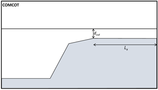
Figure 5 Numerical flume geometry with a modified profile to avoid the reflection phenomena on the x_cut position.

To attest the effectiveness of this approach, an example of the wave height propagation of a tsunami wave with H=5.6 m for T=40 min in the numerical flume is shown in Fig. 6. Figure 6a shows the propagation of the wave height in the unaltered flume with the reflection effects, and Fig. 6b shows the same propagation in the modified flume, in which the reflection effects are minimized. In the plots in Fig. 6, the x-axis is along the length of the flume, the y-axis is the time of the simulation, and the x_cut position is marked as a red line. The example wave enters the flume after 10 min (600 s) of simulation and propagates towards the coast (zero on the x-axis), reaching the x_cut position after 30 min (1800 s) of simulation. At the x_cut position, a reflected wave on the order of 1 m height is reduced by 95 %, making it possible to obtain the boundary conditions for the IH2VOF simulation. In some cases the evolution of the wave and the interaction among new tsunami waves could generate effects like standing waves. This effect is not captured by the hybrid model.

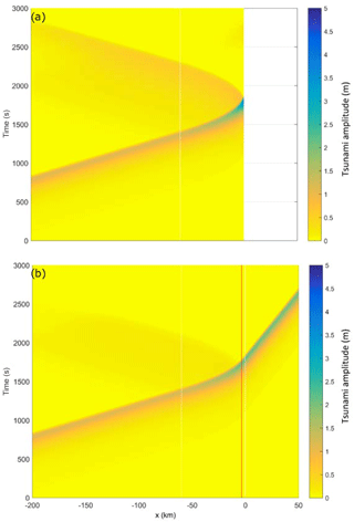
Figure 6 Propagation of a tsunami wave in the numerical flume on the distance–time plane. x_cut position is indicated on the plane with a red line. (a) In the initial domain, a reflected wave is observed, aliasing the boundary condition for the IH2VOF domain. (b) The modified domain, in which a constant infinite depth is modeled after the x_cut position. In this case, the reflection of the wave is eliminated, allowing the boundary conditions for the IH2VOF model to be obtained.

Therefore, to sum up, the procedure to simulate the propagation of a tsunami wave in the numerical flume follows the following steps: (i) COMCOT domain design based on the profile parameters and tsunami wave; (ii) COMCOT simulation to obtain a first estimate of the expected run-up; (iii) design of the IH2VOF domain, based on the run-up estimation; (iv) calculation of the position of x_cut; (v) design of the COMCOT domain inland with a modified profile to eliminate the effect of the reflected wave; (vi) COMCOT simulation to obtain the boundary conditions (input) for the IH2VOF simulation; (vii) IH2VOF simulation and (viii) run-up determination in the IH2VOF domain.

The validation of the numerical flume and the coupling of the models was made following several approaches. First, by comparing its results with the results of the physical experiments conducted by Synolakis (1987) and Baldock et al. (2009). The scenarios defined on these experiments were calculated using the IH2VOF model in order to assure that the result of the application of the exposed grid conditions (scale relation r= 5 ∕ 1) is correct. Figure 7 shows the run-up obtained in this comparison and how the results of both series of experiments fit adequately with the numerical flume results.

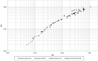
Figure 7 Validation of the numerical flume by comparing the results of its application with the results of the physical experiments of Synolakis (1987) and Baldock et al. (2009).

Additionally, due to the fact that IH2VOF model gives accurate results, the run-up calculated with the numerical flume (COMCOT + IH2VOF) was successfully compared to the result of applying IH2VOF to the whole geometry for several scenarios. Figure 8 shows a comparison among three propagations of the same scenario: (i) using IH2VOF for the whole domain, (ii) coupling two consecutive IH2VOF domains at x_cut and (iii) applying the numerical flume.

Figure 8 Comparison among the IH2VOF model and the numerical flume. Subplots of the coupling and the run-up areas are depicted.

To assess the tsunami hazard in a tsunami-prone area, this coupled model can be applied to several profiles all along the studied coastal area. The methodology provides the run-up at each of the profiles, allowing the flooded area to be estimated as an envelope of the run-up limits.

3 Application example: further development of a tsunami run-up database

The presented hybrid model was created with the aim of applying it to generate a tsunami run-up database (TRD) from a combination of bathymetric profiles and tsunami waves. The objective of this database is to create an interpolation space that allows the instant evaluation of the tsunami run-up, without needing to run numerical simulations.

This database contains the run-up of tsunami scenarios that are combinations of parameterized tsunami waves and parameterized bathymetric profiles. These scenarios have been simulated within the described numerical flume.

The following section is focused on explaining the details of the development of the TRD, the selection of the bathymetric profiles and tsunami waves and the simulations run with the hybrid numerical model. Finally, an interpolation tool, which was developed ad hoc to apply the database to the instantaneous estimation of the run-up, is presented.

3.1 TRD bathymetric profiles

The parameterization of the 50 bathymetric profiles that were selected worldwide (see Fig. 1 and Table 1) were added to the TRD. The five parameters of each of these 50 measured profiles were obtained by means of a least-squares fitting method.

To increase the number of cases included in the TRD, more realistic profiles were added as combinations of the five parameters. To generate these profiles, the ranges of the values of each parameter over the 50-profile sample set were analyzed, with a focus on identifying trends or rules that characterize their variability. The new profiles follow these trends, avoiding the inclusion of unrealistic combinations of parameters (e.g., (d₂−d₁) was always larger than 2200 m and x₁ was always shorter than 210 km). By using these realistic combinations of parameters, the TRD was expanded to 5000 profiles.

Finally, from those 5000 profiles, a selection of 49 profiles was made by means of the maximum dissimilarity algorithm (Camus et al., 2011). These 49 profiles assure a maximum variability in the profiles to further develop the TRD. The parameters of the 49 chosen profiles are given in Table A1 of Appendix A.

3.2 TRD tsunami wave parameterization

The tsunami waves for the TRD were obtained by means of simulations of realistic scenarios using the COMCOT model, applying a grid size of Δx=500 m and satisfying the CFL condition given by the model ($\frac{C\cdot \mathrm{\Delta }t}{\mathrm{\Delta }x}<\mathrm{0.5}$ where Δt is the time step of the simulation). Based on these simulations, the tsunami waves were characterized by two parameters: tsunami wave height (H) and period (T) at the depth d₂.

To generate the tsunami wave shapes with COMCOT, an infinite horizontal domain with a constant water depth was used. In the analyses of the seven focal mechanism parameters (see Sect. 2.2), some simplifications were assumed. First, to generate higher tsunami waves, the three angles were fixed to the combination that provides the maximum tsunami height, i.e., θ= 0^∘, δ= 90^∘ and λ= 90^∘. Second, D was defined in Table 2, and a width of $W=(M_o/\mathrm{6.25}\mathit{\mu }\mathit{\gamma }{)}^{\mathrm{1}/\mathrm{3}}$ is obtained by assuming a rectangular fault with proportion $L/W=\mathrm{2.5}$ and using the M₀ formulation (Table 2). Finally, Kanamori and Anderson (1977) provided a relationship between the seismic moment and earthquake magnitude: $M_{\mathrm{w}}=\mathrm{2}/\mathrm{3}\cdot \log \left(M_o\right)-\mathrm{6.07}$.

Table 2 Formulations used in the definition of the parameters of the tsunami waves included in the addition to the database.

Taking these parameters into account, the tsunami waves can be obtained in terms of earthquake magnitude (M_w), focal depth (h_focal) and water depth (d). Therefore, the influence of these three parameters on the tsunami wave height and period was explored and depicted in a general scheme in Fig. 9. As it could be intuitively expected, the higher the magnitude of the earthquake is, the higher the tsunami wave height; however, the deeper the focal depth is, the lower the tsunami wave height. On the other hand, regarding the tsunami wave period, the period increases with the earthquake magnitude or focal depth. The water depth in the rupture area affects only the tsunami period, which increases when this depth decreases.

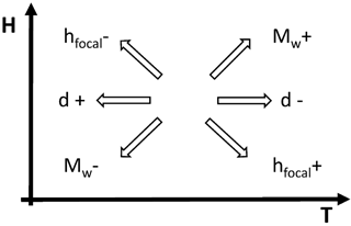
Figure 9 General scheme of the tsunami wave height (H) and period (T) behavior in relation to the water depth (d) in the generation area and earthquake focal depth (h_focal) and magnitude (M_w).

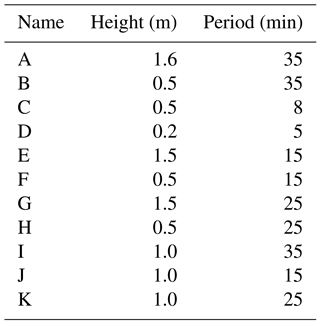
Following this characterization, a set of tsunami waves was selected, covering period values from 5 to 40 min and wave height values in the source area (depth d₂) from 0.2 to 2.0 m. In generation areas, tsunami waves are commonly within these ranges (Papadopoulos, 2016). The considered waves are peak or positive waves, meaning that the wave height was considered from the sea level. The tsunami wave heights (from A to K) and periods are given in Table 3. The interpolation is limited to the H and T ranges included in the database. The incorporation of new waves will complement the existing wave database and increase the range of application of the methodology.

Table 3 Tsunami wave height and period at the source area for the current events included in the TRD.

4 Run-up estimation by interpolation of the TRD

The procedure explained at the end of Sect. 2.4 was followed to calculate the run-up of the combination of the tsunami waves and the 49 topobathymetric profiles. Therefore, the TRD is increased by 539 scenarios, provided by seven parameters (tanβ₀, tanβ₁, tan${\mathit{\beta }}_{\mathrm{2}},d_{\mathrm{1}},d_{\mathrm{2}},H$ and T). These simulated scenarios constitute the 7-dimension interpolation domain in which new run-up calculations are carried out. The interpolation procedure and the result of its application are described next. A tool to calculate the run-up by interpolation was developed; this tool allows the simultaneous analysis of the influence of each parameter on the final value of the run-up.

4.1 The interpolation tool (IH-TRUST)

To interpolate the value of the run-up for new scenarios, a numerical tool was programmed. This tool, called Instituto Hidráulica-Tsunami Run-Up Simulation Tool (IH-TRUST), processes the profile and wave data to calculate the run-up, and it performs an interpolation of the seven parameters considered in the TRD. IH-TRUST consists of three modules, or elements (Fig. 10).

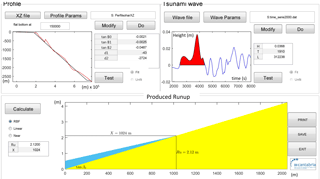
Figure 10 IH-TRUST interface, showing its three elements: the bathymetric profile, the tsunami wave parameterization and the run-up calculation.

In the first element, the tool calculates the parameterization of the real topobathymetric profile into five parameters: tanβ₀, tanβ₁, tanβ₂, d₁ and d₂. The real profile ideal trace should be parallel to the potential tsunami wave travel. The parameterization is approached by means of a least-squares fitting. An example of the fitting of a profile is shown in Fig. 11, in which the main plot shows the quadratic error in terms of distances from the coast to d₁ (X₁) and to d₂ (X₂), and the star indicates the minimum error, which is consequently the position of the best set of five parameters. The subplot shows the original profile and the parameterized profile. Afterwards, the tool verifies that the parameterized profile is included in the ranges of the parameter values contained in the interpolation space.

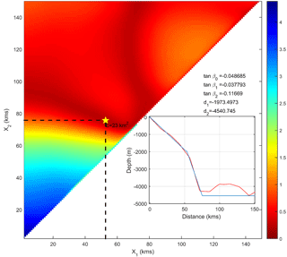
Figure 11 Parameterization of the bathymetric profiles. The figure maps the E_rms values as a function of the distance from the coast to d₁ (X₁) and the distance from the coast to d₂ (X₂) obtained during the process of finding the best parameters for a profile. In the subplot, the original profile and the parameterization are shown.

Figure 12 shows a representation of all the profile domains in black and the introduced profile in red. A set of bars indicates the acceptable values for each parameter, and a star marks the position of each parameter for the new profile.

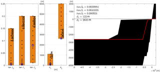
Figure 12 Fitting of a topobathymetric profile in the TRD. Each parameter value (left) and parameterized profile shape (red) for the profiles are included in the TRD (black).

In the second element, IH-TRUST calculates the values of the amplitude and the period of the tsunami wave at depth d₂. The tool reads a time series containing the tsunami shape and calculates H and T. T corresponds to the time between the first two zero crossings for positive heights, and H is the maximum positive amplitude observed within period T. The tool allows manually setting the height and period within the time series (Fig. 13). This is especially useful when the wave shape is not standard, the wave has a leading depression or it is not the largest wave of the series.

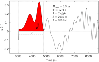
Figure 13 Tsunami wave profile parameterization in the IH-TRUST tool, including the part of the tsunami time series considered (in red) to calculate the period T and the height H.

After the wave parameters are calculated, IH-TRUST checks if the tsunami wave fits in the interpolation domain of the database. Figure 14 shows the tsunami waves included on the database, the area where the interpolation is valid and the position of the tsunami wave that is being studied.

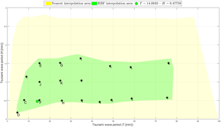
Figure 14 Tsunami wave height and period cases included in the database. The point corresponding to any new wave should fall in the green shadow in order for it to be able to be interpolated with the generated TRD.

Finally, in the third element of IH-TRUST, the results of the calculation of the run-up Ru is given based on the profile parameters and the tsunami wave. The interpolation (Fig. 10) is calculated by means of the RBF (Camus et al., 2011) and linear and nearest interpolation methods. In addition, the horizontal flooding distance X is calculated using the inland slope. The tool uses an RBF interpolation by default, but the nearest or linear methods are also available, as they are useful in calculating events that plot closer to the boundary of the valid interpolation area.

4.2 Influence of the profile parameters on the tsunami run-up

The TRD and IH-TRUST were used to explore and analyze the influence of each parameter of the profile on the final value of the run-up. This analysis was approached by evaluating scenarios in the TRD. Although it is out of the scope of this paper, to understand the influence of each parameter of the bathymetric profile, several tests were conducted with a mean profile (tanβ_0 m= 0.080, tanβ_1 m= 0.09, tanβ_2 m= 0.110, d_1 m= 500 and d_2 m= 4350) and by varying only one of the five parameters that define the profile at a time; additionally, several values of H and T inside the boundaries of the domain were considered.

For each pair of values of H and T, four of the five profile parameters were kept constant, and the run-ups were calculated using IH-TRUST with the TRD by varying the 5th parameter.

The effect of the variation in Ru / H as a function of the parameters are shown in Figs. 15 and 16.

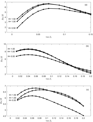
Figure 15 Maximum run-up (normalized by wave height) as a function of the profile slopes (tanβ₀, tanβ₁ and tanβ₂) of the parameterized profiles for different wave heights.

The continental slope effect (Fig. 15), parameterized as tanβ₂, produces a maximum Ru when tanβ₂ is close to tanβ₁, reproducing a single slope profile. For smaller tanβ₂ values, Ru decreases rapidly due to wave shoaling. Low values of tanβ₂ also indicate a large platform with a low slope, where the shoaling increases the wave height and the wave energy diminishes gradually due to bottom friction until wave breaking occurs. Thus, the energy flux that reaches the shore decreases with the run-up height. The profile typology characterized by a low value of tanβ₂ is closer to Synolakis's canonical problem.

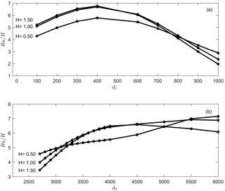
Figure 16 Maximum run-up heights as a function of the profile slopes (d₁ and d₂) of the parameterized profiles for different wave heights.

The higher the tanβ₂ is, the shorter the platform, reducing the energy dissipation and allowing the slopes to have similar tanβ₀ and tanβ₁; this maximizes the run-up height.

Regarding tanβ₁, when d₁ is constant (Fig. 15), the higher tanβ₁ is, the shorter the length of the shelf, reducing tsunami wave shoaling. In this case, the wave steepness increase drastically near the coast and breaks abruptly, triggering a considerable dissipation of energy within a short length; this effect reduces both the energy flux on the coast and the run-up.

Kânoğlu and Synolakis (1998) show that in the case of solitary waves the slope closest to the coast controls the run-up processes. In the case of tsunamis, in our geometry, although the influence of tanβ₁ is indeed important, the influence of tanβ₂ must not be neglected.

Finally, the influence of tanβ₀ on the final value of the run-up is less important than those of tanβ₁ and tanβ₂. The run-up decreases as tanβ₀ increases. Due to the effect of gravity, the flow ascends less if greater slopes are present. This aspect is strengthened by the reflection of the energy.

The behavior described above can be summarized on three basic regimes, depicted in Fig. 17: (i) the larger run-up for any wave height is found if tanβ₁ = tanβ₂ (see Fig. 17b); (ii) when tanβ₁ > tanβ₂ see Fig. 17c, the bigger the difference between slopes, the smaller the run-up, mainly because the increase of dissipation; and (iii) when tanβ₁ < tanβ₂, see Fig. 17d, the run-up is also smaller, but in this case it is due to the effect of increasing reflection.

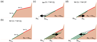
Figure 17 Influence of the variation of the tanβ₁ and tanβ₂ on the run-up. Panel (a) shows a scheme of the profile where segment of tanβ₂ is marked as green and tanβ₁ as red. Panel (b) shows the situation where tanβ₁ = tanβ₂. Panel (c) depicts the situations where tanβ₁ is larger than tanβ₂. And, finally, panel (d) shows the situations where tanβ₁ is smaller than tanβ₂.

The influence of depths d₁ and d₂ is shown in Fig. 16. For deeper continental shelf depths d₁, the shelf is wider and, consequently, the bottom friction affects the wave over a longer profile, creating a smaller run-up. For a constant tanβ₁, lower values of d₁ represent a shorter continental shelf, and abrupt and dissipating wave breaking. Moderate values of d₁ are characterized by a gradual tsunami wave shoaling, during which the bottom friction allows a maximum run-up. From that critical point, higher values of d₁ mean a longer continental shelf, generating a larger frictional area, reducing the energy flux that reaches the shore and consequently diminishing the run-up.

In Fig. 16b, it can be observed how the run-up increases almost linearly with d₂. The effect of d₂ in the run-up is similar to the effect of tanβ₂. The shallower d₂ is, the greater the shoaling and the higher the wave. The wave energy diminishes gradually due to bottom friction until wave breaking, which depends on the tsunami wave height. In addition, it was found that although the variations in wave height produce different Ru / H values for the same profile, the influence of the variation in the wave period is negligible. Therefore, different wave heights but not different periods are shown in Figs. 15 and 16.

Finally, these results highlight the importance of using an accurate geometry to define the run-up. The influence of d₂ and tanβ₂ in the final run-up estimation is considerable, and the use of complete profiles, from the generation area to the coast, is necessary but not considered in traditional approaches and simplifications.

5 Validation of the methodology with numerical test results and observational data

The methodology presented here aims to calculate the tsunami run-up in coastal areas. This calculation can be applied to study the run-up of historic events but also to calculate the run-up of potential scenarios, which are the primary focus. These potential cases are used to evaluate tsunami hazard and the flooded area when a tsunami occurs. As mentioned in the introduction, run-up is commonly assessed by means of high resolution data.

Therefore, to validate this methodology or tool, the results of its application have been compared with both high-resolution numerical simulations of potential events and historical tsunami run-up scenarios. It is important to highlight that the presented tool allows the estimation of tsunami run-up when these HR data are not available or accessible, what is a common situation.

The results of these comparisons are detailed in the following subsection, which is focused on describing the strengths and limitations of the methodology for each case.

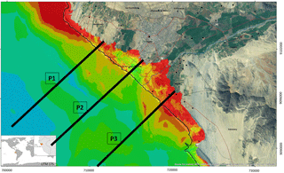
Figure 18 Flooded area in the municipality of Trujillo in Peru, due to a tsunami triggered by an 8.5 magnitude earthquake, including three selected profiles with the run-up obtained by using the numerical model. The coordinates of the exact locations where the run-up was estimated are provided in Table 4.

5.1 Validation with numerical model simulations

This validation was carried out as follows: first, a topobathymetric profile of the study area was obtained using the GEBCO database. On that profile, a point was selected offshore, and the time series of the tsunami was extracted at that point from the COMCOT numerical simulation of the event. Using the topobathymetric profile and the time series as input for the IH-TRUST tool, the run-up was interpolated by using the created database. The interpolated run-up was then compared to the run-up obtained by using the high-resolution numerical simulation of the potential scenario.

Three numerically simulated scenarios with high resolutions have been selected for the validation. All these scenarios are from real projects, studies and published papers that were focused on analyzing and assessing the tsunami hazard in coastal areas worldwide and characterizing the potential flooded areas due to tsunami events in the selected zones. These simulations used high-resolution topographic and bathymetric data to construct grids with 30 m cells.

5.1.1 Tsunami scenario in Trujillo, Peru

The results of the application of the methodology were compared to the results of a high-resolution numerical simulation of a magnitude 8.5 event in the subduction zone located along the coast of Trujillo, a municipality in northern Peru. This synthetic scenario represents the event that occurred in this zone in 1619 and is part of the study “Probabilistic evaluation of the hazard and vulnerability under natural disasters in the metropolitan area of Trujillo”, funded by the Inter-American Development Bank (IHCantabria, 2013). The numerical simulation used a 30 m-resolution grid to accurately calculate the flooded area for a tsunami wave height and period of approximately 1.5 m and 400 s at a depth of 3000 m.

In Fig. 18, the flooded area map of Trujillo, as well as the selected profiles, are shown. In the study, the numerically calculated run-ups at those profiles (Fig. 19) were 8.9, 10.6 and 12.8 m. The corresponding values for the run-up obtained by interpolating the TRD with the IH-TRUST tool were 8.8, 10.5 and 11.6 m (see Table 4). Compared to the results of the numerical simulation, these 3 values from the 3 zones of the study area provide a good approximation of the tsunami flooding.

Figure 19 Topobathymetric profiles selected in Trujillo, Peru to validate the methodology. The topobathymetric profile (blue) and the parameterized profile (red) are compared.

5.1.2 Tsunami scenario in La Libertad, El Salvador

Following the same procedure, a validation case was addressed in El Salvador. The event is a potential scenario of an earthquake of magnitude 8.1 along the El Salvador thrust, which is in the subduction zone along the El Salvador coast. The study area is the flat area of La Libertad, on the western side of this Central American country. This high-resolution numerical simulation is part of the project “Tsunami Risk Assessment in El Salvador”, financed by AECID (Spanish Agency for International Cooperation and Development) during the period 2009–2012 (Álvarez-Gómez et al., 2013). The resolution of the numerical simulation was 30 m, and the grid that was built for the propagation and inundation calculations used data from local bathymetric campaigns and high-resolution topographic studies. The tsunami wave height and period at a depth of 3000 m were approximately 0.9 m and 700 s.

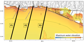
Figure 20 Flooded area in the municipality of La Libertad in El Salvador, due to an 8.1 magnitude event with epicenter along the coast of this Central American country. The exact locations where the run-up was estimated are provided in Table 4.

In Fig. 20, the flooding map that was part of this project is shown, and in the same figure, the selected profiles have been superimposed. In this simulation, the run-ups obtained at the three profiles in Fig. 20 were 5.2, 5.5 and 6.3 m. The corresponding run-ups obtained by interpolating the TRD with the IH-TRUST tool were 6.2, 6.1 and 7 m.

5.1.3 Tsunami scenario in Muscat, Oman

As part of the Multi Hazard Risk Assessment System of Oman (Aniel-Quiroga et al., 2015), more than 3000 potential tsunami events were numerically modeled. A selection of these events were selected to assess the tsunami hazard for some specific municipalities in Oman by means of high-resolution numerical simulations of the generation, propagation and inundation processes, with a 30 m grid. One of these cases was an extreme event of magnitude 9.0 with epicenter in the Makran Subduction Zone (MSZ). For the capital city area, Muscat, the resultant flooding map is shown in Fig. 21; the profiles that were selected for the validation are superimposed on this map. The tsunami wave height and period offshore were approximately 2 m and 2300 s. In these cases, the measured run-ups at each profile were 6.2, 8.7, and 7.7 m. The corresponding run-ups calculated with the new database were 6.3, 8.5 and 7.8 m.

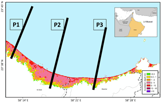
Figure 21 Flooded area in the municipality of Muscat, capital city of Oman, due to a 9.0 magnitude event with epicenter in the Makran Subduction zone. The extracted locations where run-up was estimated and the run-up values, both modeled and estimated with the IH-TRUST tool, are provided in Table 4.

Table 4 summarizes the results obtained for the validation with the high-resolution simulations in the three scenarios. The run-up values, both those calculated with the numerical model and those estimated with the proposed database and detailed methodology described above, have a similar magnitude; in some cases, the result is accurate enough to rely on the results of the presented methodology. In addition, in Table 4, the estimated run-up is also compared to the result of applying 2 empirical run-up formulae. First, the Synolakis formula, that although it was created for the run-up of solitary waves, has been widely applied in the past for tsunamis, and second, the Madsen and Schäffer expression for single waves (Madsen and Schäffer, 2010). In the application of this expressions an averaged slope was considered.

Table 4 Tsunamis scenarios included in the validation process of the database and tool. The numerical model column includes the run-up obtained with the high-resolution numerical simulations and can be compared to the estimations from the application of the IH-TRUST and formulae of Synolakis (Synolakis, 1987) and Madsen and Schäffer (2010).

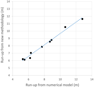
Figure 22 shows this comparison in a plot, in which the fitting between the modeled and calculated run-up values is noted. In addition, the new methodology is better than the result of the Synolakis and Madsen and Schäffer formulae, which generally overestimates the run-up.

Figure 22 Plot of the numerically modeled run-up against the calculated run-up values for the validation cases.

5.2 Validation with data recorded during field campaigns after real events

The low frequency of major tsunamis are invaluable to the field campaigns that are carried out immediately after a tsunami event occurs. These field campaigns allow the evaluation of the developed strategies of risk reduction and the creation of new, more accurate strategies. From a pragmatic point of view, the data collected during these campaigns allow scientists and engineers to validate or calibrate numerical models and methodologies. In this case, this type of validation has been addressed using the available field data of the events in Japan (2011) and Chile (2010 and 1960). The bathymetric profiles used in the validation have been constructed using GEBCO. The tsunami wave time series have been obtained from the data available from DART buoys (Meinig et al., 2005) or numerical simulations of accurate sources; this process is explained in detail later in the paper. The results of the application of the methodology have been compared to observational data recordings and field survey papers.

5.2.1 2011 tsunami on the coast of Japan affecting the Pacific basin

On the 11 March 2011, a 9.0 earthquake, which had an epicenter close to the coast of Japan, triggered a tsunami that reached the coast of Japan within one hour. This tsunami wave propagated across the Pacific Ocean, reaching the U.S. West Coast in 10 h and the coast of Chile in 21 h.

The tsunami wave time series used for this validation have been obtained from the data available from DART buoys (Meinig et al., 2005). The results were compared with the observed run-up (National Geophysical Data Center NOAA).

It is essential to highlight that the application of the new run-up estimation methodology is restricted to the profiles and wave shapes whose parameters fall inside the ranges covered by the database (see Table 1). Therefore, the use of the methodology is limited to these cases. An example of non-applicability occurs when the tsunami height and period are obtained (d₂) in a shallow area of the ocean or when the generation zone is too close to the study area and a complete time series of the tsunami wave cannot be properly recorded at an adequate depth.

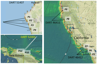
Figure 23 Validation with DART buoy time series. 4 DART buoys were used, and their data were applied to several bathymetric profiles to validate the methodology. The locations of the points where the run-up was estimated are included in Table 5.

In the case of the Japan 2011 event, due to the proximity of the coast, it was not possible to obtain a complete time series between the epicenter and Japan, and the validation has been carried out in other areas of the Pacific Ocean, using four DART buoy records (near Hawaii, California, and Papua-New Guinea). The names and locations of the DART buoys used are given in Table 5. This table also includes the names and locations where the run-up was estimated with the data of each DART buoy, the run-up value recorded in the field surveys at those locations, and the estimated value of the run-up, both by using the new methodology and by applying the Synolakis formula (calculating the tsunami wave height at a depth of 10 m using Green's law) and Madsen and Schäffer formula. The buoy locations are also included in Fig. 23.

Table 5 Validation with DART buoy time series of the Japan 2011 event. 4 DART buoy datasets were used on several bathymetric profiles to validate the methodology. Location names correspond to those given by the National Geophysical Data Center (NOAA). Synolakis run-up was estimated by applying the so-called Green's Law to the time series of the DART buoys to obtain the tsunami height near the coast.

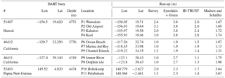
As it can be inferred from the application of the methodology, the run-up estimated values are on the same order of magnitude as the recorded inundation; generally, the results are accurate, and differences are normally lower than 20 %. These results are also closer to the observed run-ups than those obtained by applying Synolakis and Madsen and Schäffer formulae, which often overestimates the run-up.

5.2.2 Chilean coast tsunamis (2010 and 1960)

When no real record is available to determine the offshore wave shape (DART buoys), the main issue is the correct definition of the source to compute an accurate numerical simulation. Although there is no shortage of uncertainties in the determination of the source, the tsunami initial surface deformation models that have been developed are accurate (Barrientos and Ward, 1990). As an alternative validation approach, two of these models have been used to validate the new run-up estimation methodology with the events that occurred in Chile in 2010 and 1960.

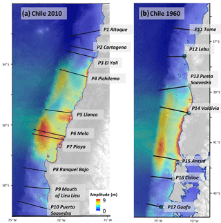
Figure 24 Profiles and locations used in the validation of the new methodology by using the run-up recorded after the tsunami events of 2010 (a) and 1960 (b) in Chile. The locations of the points where the run-up was estimated are included in Table 6.

Table 6 Validation of the methodology with the results of numerical simulations of realistic sources of the 1960 and 2010 events on the coast of Chile. Fritz et al. (2011) survey results were used to validate the results from the new methodology for the Chile 2010 event. NOAA's National Geophysical Data Center data were used to carry out the comparison with the 1960 event.

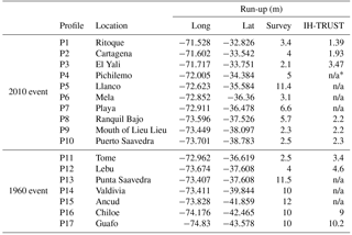
^*n/a = Not applicable.

On the 27 February 2010, an 8.8 magnitude earthquake with epicenter on the coast of Chile triggered a tsunami that reached the Chilean coast in less than 30 min. In the Bio-Bio region, the run-up was recorded at several locations (Fritz et al., 2011). To apply this methodology, first, a rough numerical simulation of the generated tsunami was addressed. This simulation used the source definition by Shao et al. (2010) and gridded the GEBCO data with 700 m cells (see Fig. 24). From this simulation, the profiles and wave amplitude time series in the generation area were obtained. The tsunami wave height and period recorded at each location and the result of the interpolation from the further improved database for each corresponding profile are given in Table 6.

The optimal application of the run-up estimation methodology is achieved at the locations sufficiently far from the source, as explained in the previous subsection. The result at these points (1, 2, 3, 8, 9 and 10) have the same order of magnitude of the recorded run-up from Fritz's survey. In the locations in front of the source, the initial deformation of the water surface did not allow a complete time series to be obtained to estimate the tsunami wave height and run-up.

Regarding the 1960 earthquake and tsunami in Chile (Lomnitz, 2004) (Fig. 24), this earthquake is considered the greatest earthquake ever recorded, and the numerical simulation computed for the validation used the source by Barrientos and Ward (1990). The run-up data for the validation was obtained from the NOAA global historic tsunami database. In this case, the data are mainly from eyewitness testimony.

In Table 6, the results of the application of the methodology at seven locations and the recorded run-up are given. In this case, the tsunami wave height at three of the locations (P13, P14 and P15), was such that the profiles were not within the database application ranges. The other four locations provided results that are on the same order of magnitude as the observed run-up.

In the application of the new methodology to the Chile events, the tsunami wave height used for the interpolation came from a numerical simulation, and the results were compared to real run-up records. Although the validation inherits the uncertainties of the source, the results are sufficiently accurate, taking into account the limitations explained above.

6 Conclusions

The calculation of the flooding that a tsunami causes inland is addressed when a tsunami risk assessment is conducted. For a historical event, the assessment determines the limit of the affected area. In addition, the predictive evaluation of this flooded area, based on the potential tsunami scenarios that can affect it, allows prevention and mitigation measures to be established, helping to reduce the risk.

However, the calculation of this flooded area, particularly the assessment of the run-up, is not always direct. Occasionally, there are no high-resolution data that allow the application of numerical models. In addition, the accuracy of the existing empirical formulae can be improved, since they do not take into account natural topobathymetric profiles from the propagation to the inundation areas.

In this paper, an alternative methodology that complements the existing ones has been presented. This methodology consists of a numerical flume formed by the coupling of two numerical models (COMCOT and IH2VOF). The developed hybrid model is applied to each part of the generation–propagation–inundation process and this numerical model obtains a more accurate result; additionally, it is computationally affordable. The inputs for this hybrid model are the topobathymetric profile and the tsunami wave. The topobathymetric profiles were parameterized with five parameters (three slopes and two depths), using a real profile sample to define the parameterization. In addition, the tsunami waves were parameterized with two parameters (tsunami height and period) using tsunami amplitude time series obtained by using numerical simulations of realistic tsunami events.

This methodology allows the accurate calculation of the run-up on along topobathymetric profile. Therefore, this methodology has been used to construct a tsunami run-up database. This database aimed to create an interpolation domain in which new run-up calculations could be carried out. The events of the database are combinations of a selection of bathymetric profiles and tsunami waves that were simulated with the hybrid model to create the database of simulations from which an interpolation can be executed to calculate the run-up of new tsunami scenarios.

To easily address the interpolation, a tool called IH-TRUST was scripted. This tool uses real profile and wave data, parameterizes them to find their most similar parameters in the database, and interpolates the results to provide a run-up value. Once the input parameters are given, the application of this interpolation provides results in just a few seconds, shortening typical simulations of several nested grids, which commonly take several hours to provide results in all the computational domain.

To validate this new methodology and tool, the results of its application have been compared with both high-resolution numerical simulations and field survey data. The run-ups obtained with IH-TRUST are consistent and suggest that the tool can accurately calculate the run-up.

The assessment of the tsunami hazard begins by calculating the area affected by the tsunami. In those coastal areas where no other data are available, the detailed methodology and tool allow the run-up value of tsunami events to be determined without using high-resolution numerical simulations.

Therefore, to assess the hazard in a tsunami-prone area, this methodology can be applied to several profiles along the coastal area study. As a result, the methodology provides the run-up at each of the profiles, allowing an estimation of the flooded area from an area within the envelope of the run-up limits.

The application of the tool has some limitations; for example, the tool will indicate if the bathymetric profile or the tsunami wave parameters are not included within the range of values in the database, as explained for the case of the Chilean Trench in Sect. 5.2.1.

New work in this field should take into account these difficulties to further develop the database with new parameter values that include these singularities.

The generation of the database and the values of run-up obtained from a combination of the bathymetric profiles and tsunami waves have provided a rich and populated space where the influence of each parameter on the final value of the run-up can be addressed. In this sense, which profiles are more prone to suffer higher run-ups in the case of a tsunami can be defined. For instance, profiles with high land slopes (tanβ₀) are associated with higher run-up values than those with low land slopes. In addition, some combinations of offshore slopes and continental shelf slopes (tanβ₁ and tanβ₂) minimize the run-up value for the same tsunami wave. In addition, the influence of tanβ₂ is considerable and justifies inclusion of the deep-water area (d₂) in the parameterized profile. Conversely, when the profile is for a large continental shelf, the run-up increases; however, the run-up value decreases for gentle continental shelf slopes.

Traditionally, empirical methods, like the application of Synolakis's formula, simplify the profile using one or two slopes (Park et al., 2015). However, this assumption is not accurate; in this study, the importance of using a complete profile, including the tsunami generation area, has been noted, as well as the influence of the profile parameters on the final run-up value.

Appendix A: Database profiles

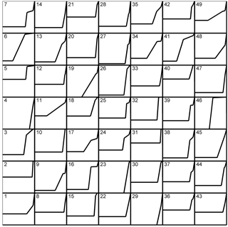
In this section, the 49 artificially generated profiles are shown in Fig. A1. The five corresponding parameters are listed on Table A1.

Figure A1 The 49 profiles used to generate the IH-TRUST database.

Table A1 Synthetic profiles.